OVERVIEW
In a previous blog of our series of blog articles illustrating Rjags programs for diagnostic meta-analysis model, we looked at how to carry out Bayesian inference for the Bivariate model as well as the Bivariate model when a perfect reference test is not available, e.g latent class model.
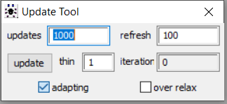
In this blog article, we will revisit both Bivariate models to explore what can be the consequences on the model’s parameter estimates of ignoring the Adaptation incomplete warning that can come up at the model compilation step like this :

MOTIVATING EXAMPLE AND DATA
For our motivating example we will once more use the data from a systematic review of studies evaluating the accuracy of GeneXpertTM (Xpert) test for tuberculosis (TB) meningitis (index test) and culture (reference test) for 29 studies (Kohli et al Kohli et al. (2018) ). Each study provides a two-by-two table of the form
| reference_test_positive | Reference_test_negative | |
|---|---|---|
| Index test positive | t11 | t10 |
| Index test negative | t01 | t00 |
where:
t11is the number of individuals who tested positive on both Xpert and culture testst10is the number of individuals who tested positive on Xpert and negative on culture testt01is the number of individuals who tested negative on Xpert and positive on culture testt00is the number of individuals who tested negative on both Xpert and culture tests
BAYESIAN AND MCMC CONCEPTS
In the context of the motivating example discussed above, the Bayesian approach consists of updating any prior belief (Expert opinions if available, vague priors otherwise) we have on the sensitivity and specificity of both Xpert and culture tests with each 2x2 tables provided by the studies of the meta-analysis (the data) to draw a posterior conclusion about both Xpert and culture test propertises.
The Markov Chain Monte Carlo (MCMC) methods are tools that allow sampling from a probability distribution via iterative algorithms. The algorithm consists of building a Markov chain that in the limit as the number of iterations approaches infinity, will have the desired distribution as its stationary distribution.
By joining the two concepts together, we will express our prior belief as prior probability distributions, that will later be updated by the 2x2 tables of data provided by the studies to form the posterior distributions of sensitivity and specificity of both tests.
In practice the iterative algorithm will have a finite number of iterations giving us access to a sample of the posterior distribution. The algorithm will be divided into two parts : An adaptavie/burn-in period during which every iteration will be discarded, followed by the actual sampling of the posterior distribution which consists of iterations that are considered to have converged sufficiently close to the stationary distribution we are trying to approximate.
ADAPTATION VS BURN-IN
In rjags, the adaptation phase is performed before the burn-in step when the model is compiled with jags.model function. It’s default value is set to n.adapt=1000. It is a period during which the algorithm will tune up its own parameters in order to later generate samples as efficient as possible.
The burn-in part, which will occur after the adaptation step, is usually regarded as a period where the iterations have not converged yet, e.g. the resulting sample draws are not sufficiently close enough to the stationary distribution to reasonably estimate it. This sometimes happens if initial values were selected far from the center of the distribution. Keeping those burn-in iterations could potentially bias the final estimates.
WHAT IS THE ISSUE?
The JAGS manual (section 3.4) recommands running adaptation phase in order to optimize the sampling algorithm, even suggesting to start from scratch using a longer adaptation period if a given n.adapt failed to prevent the warning. It seems to be the case in JAGS that some complex models tend to trigger the Adaptation Incomplete warning even for large number of n.adapt values.
This made us wonder what would actually happened if we just ignored the warning and proceed with the burn-in and sampling steps? In other words, what would be the impact on the posterior distribution estimates of running the sampling algorithm with a sub-optimal sampler? In order to try to answer that question we will first study the impact of varying the n.adapt value on the Bivariate model and then on the more complex Bivariate latent class model.
BIVARIATE META-ANALYSIS MODEL
The bivariate model assuming culture test is a perfect reference test is a much simpler model than the one that assumes culture is imperfect. We will therefore run this model with different values of n.adapt in an attempt to have one model where the warning was triggered and one model where it was not. Then we will compare the parameter estimates of both models that will basically be identical except for the number of n.adapt iterations ran during the adaptation phase. Our goal will therefore be to study what is the impact of the Adaptation incomplet warning message on the estimation of the parameters of the model.
We will also look at convergence statistics, Rhat and n.eff. The former is is the Gelman-Rubin statistic (Gelman and Ruben(1992), Brooks and Gelman(1998)). It is enabled when 2 or more chains are generated. It evaluates MCMC convergence by comparing within- and between-chain variability for each model parameter. Rhat tends to 1 as convergence is approached. The latter is the effective sample size (Gelman et al(2013)). The MCMC process causes the posterior draws to be correlated. The effective sample size is an estimate of the sample size required to achieve the same level of precision with a simple random sample. If draws are highly correlated, the effective sample size will be much lower than the number of posterior samples used to calculate the summary statistics.
BIVARIATE MODEL WITH OPTIMAL SAMPLING BEHVIOR
We first decided to run the default n.adapt=1000 argument unchanged.
jagsModel = jags.model("model.txt",data=dataList,n.chains=3,n.adapt=1000)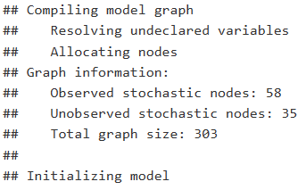
It turns out that this model does not trigger the Adaptation Incomplete warning. According to JAGS manual, this means the sampler managed to tuned its parameters in such a way that the sampler has converged to their optimal sampling behavior.
The complete specifications of the model are as followed. We run a 3-chain model with :
- Adaptation phase of
1000iterations - Burn-in phase of
15000iterations - Draw
100000more iterations with a thinning value of10to estimate the posterior distribution of each parameter with a posterior sample of10000iterations for each chain
This mean that our final posterior sample for each parameter will consist of 30000 iterations. Let’s first look at the parameter estimates of the Bivariate model when the warning does not trigger.
# Summary statistics
output_1000 <- read.table("output_1000.txt",header=TRUE)
colnames(output_1000)[4:6] <- c("2.5%", "50%", "97.5%")
datatable(output_1000, extensions = 'AutoFill', options = list(autoFill = TRUE))
In a meta-analysis context where the goal is to evaluate the diagnostic accuracy of the (Gene)Xpert test, we find that the summary sensitivity (Summary_Se) and summary specificity (Summary_Sp) of Xpert are estimated to be 71.02% [95% credible interval : 60.77 - 80.27] and 98% [95% credible interval : 96.92 - 98.81], respectively. In terms of convergence, they both have a Gelman-Rubin statistics of Rhat= 1. Further more, their effective sample size are n.eff= 16976 and n.eff= 15329, respectively. This mean that despite the posterior estimates being based on a sample of size 30000, we can consider that roughly half of it equivalent to a simple random sampling where there are no auto-correlation among successive draws.
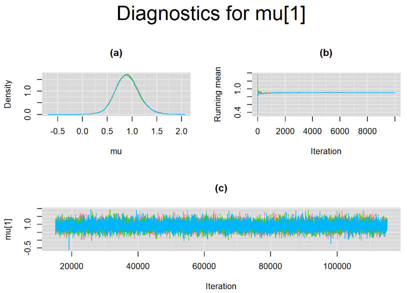
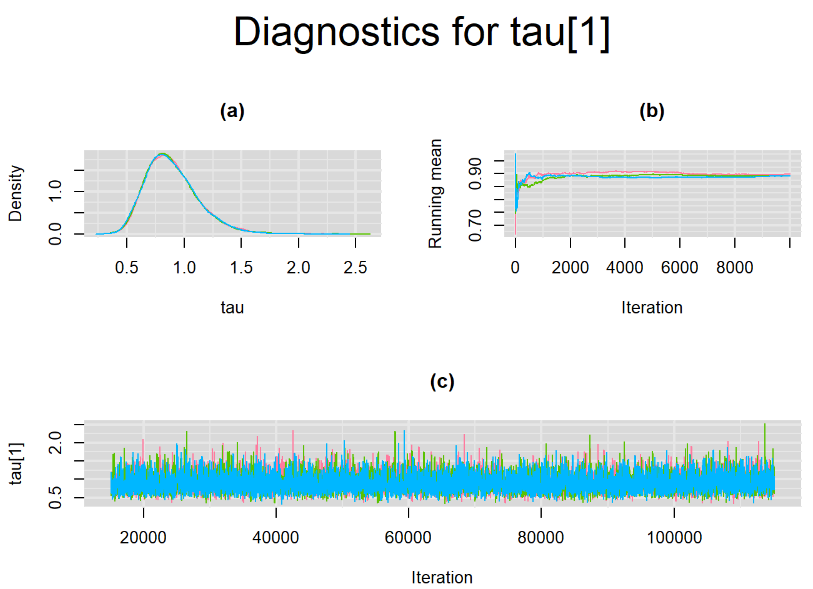
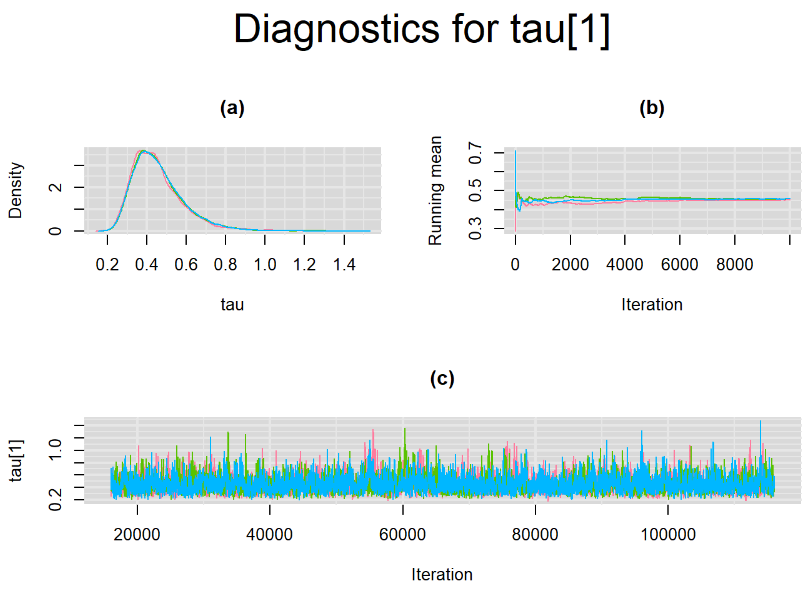
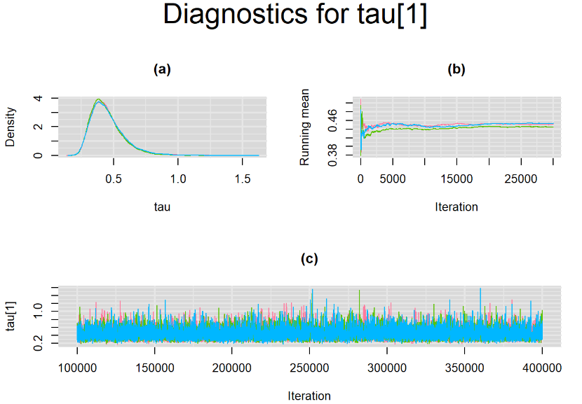
Every other parameters have a Gelman-Rubin statistic of 1. All parameters have effective sample size equals to at least a third of the 30000 posterior sample size, except the between-study standard deviation parameters (tau[1] and tau[2]),
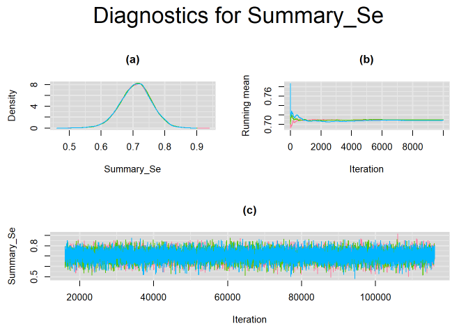
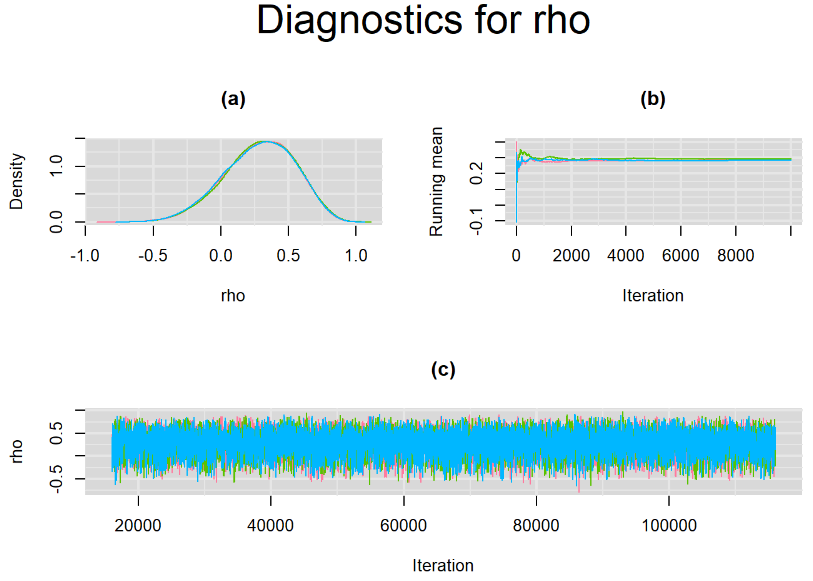
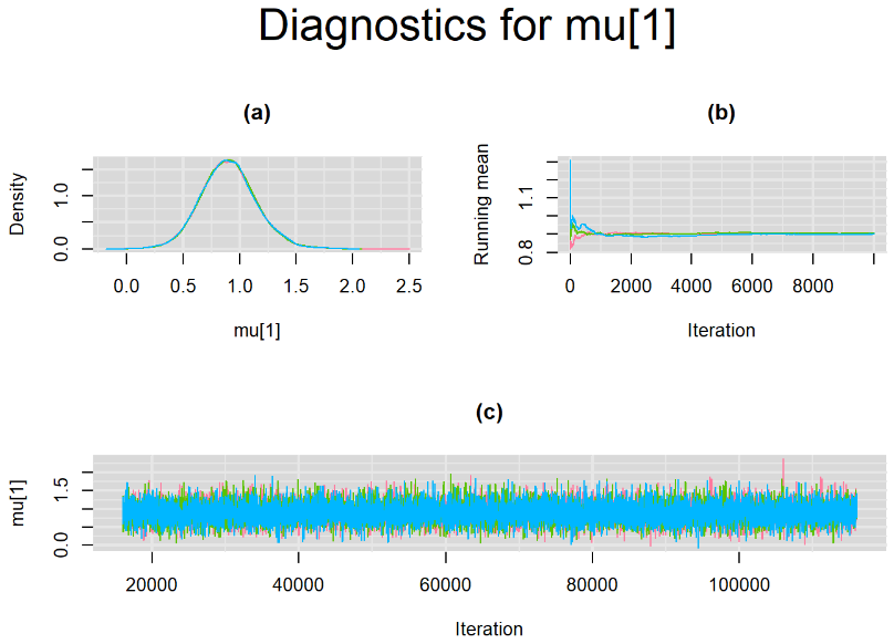
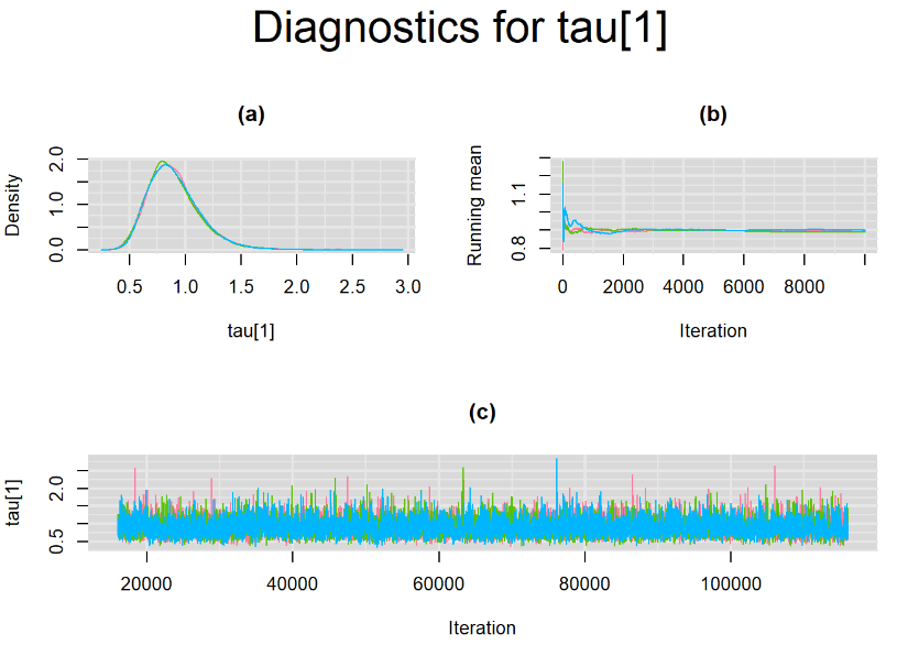
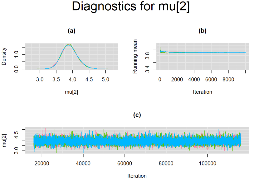
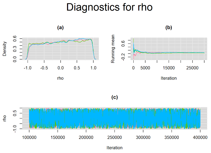
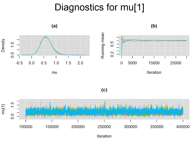
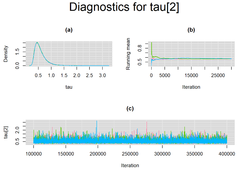
Since, it is always good practice to accompany convergence statistics with a plot, we present density, trace and running mean plots for some key parameters of the model, including tau[1] and tau[2]. No parameter shows any sign of convergence issue, we would therefore conclude that this model has converged and we would be confident toward the posterior parameter estimates.
BIVARIATE MODEL WITH NON OPTIMAL SAMPLING BEHVIOR
Keeping the same bivariate model with the same settings discussed in the previous section, e.g. we run a 3-chain model as follow :
Burn-in phase of
15000iterationsDraw
100000more iterations with a thinning value of 10 to estimate the posterior distribution of each parameter with a posterior sample of10000iterations for each chain
This mean that our final posterior sample for each parameter will consist of 30000 iterations.
But this time, we were able to trigger the Adaptation Incomplete warning by running an insufficient number of n.adapt iterations. For instance, fixing n.adapt=100 did trigger the warning.
# Compile the model
jagsModel = jags.model("model.txt",data=dataList,n.chains=3,inits=Listinits,n.adapt=100)
In that instance, the parameter estimates obtained from the model are as follow:
# Summary statistics
output_100 <- read.table("output_100.txt",header=TRUE)
colnames(output_100)[4:6] <- c("2.5%", "50%", "97.5%")
datatable(output_100, extensions = 'AutoFill', options = list(autoFill = TRUE))
We can see that running the model with sufficient sample size did not change the posterior estimates, aside from sampling random error. Among others, the mean sensitivity (Summary_Se) and mean specificity (Summary_Sp) of Xpert are very close to the previous estimates, this time with 71% [95% credible interval : 60.91 - 80.22] for Summary_Se and 98% [95% credible interval : 96.93 - 98.8] for Summary_Sp. Once more, every parameter have a Rhat= 1. Once again, the effective sample size are n.effare equals to at least a third of the 30000 posterior sample size except for the between-study standard deviations.
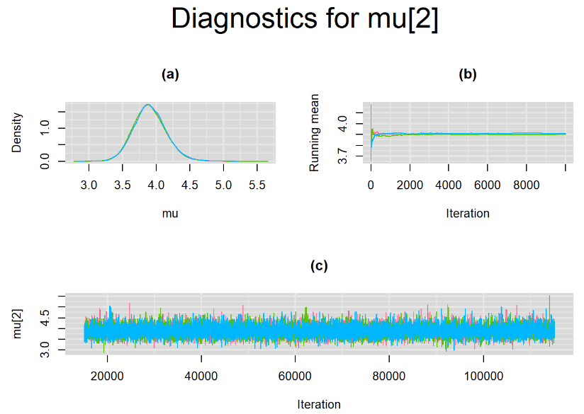
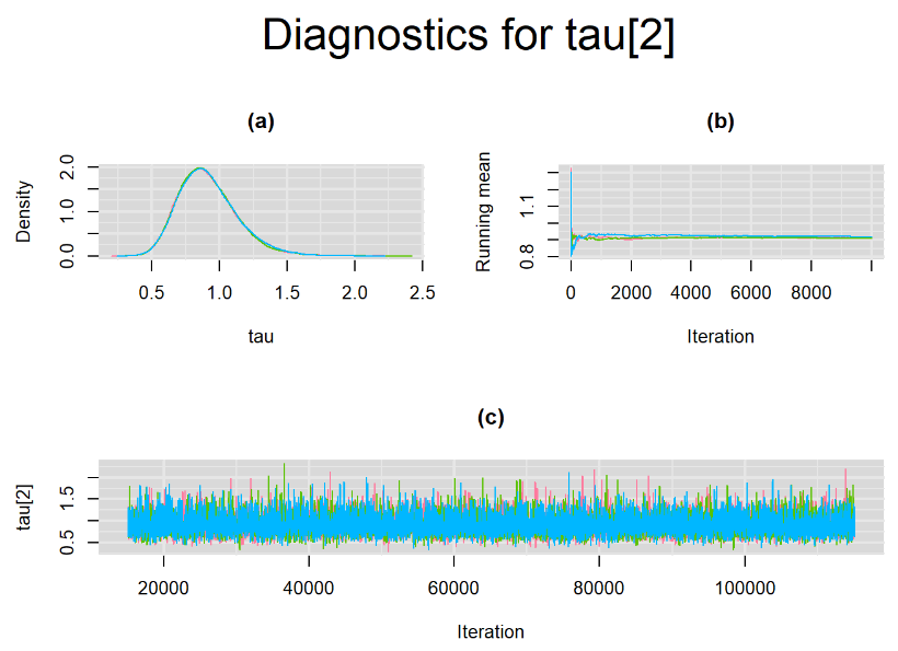
Graphically, there is nothing suspicious with the density, trace and running mean plots of the parameters below. Therefore in this example, the impact of the sampler not having reached its optimal behavior seems marginal, suggesting this warning could actually be ignored.
BIVARIATE LATENT CLASS META-ANALYSIS MODEL
In this section the bivariate model was modified as we have seen in a previous blog article in order to account for the imperfect nature of the culture test. Our goal was to aimed at repeating what was done in the previous section but after replacing the Bivariate model assuming the culture reference test is a perfect test by the Bivariate latent class model that allows the culture reference test to be an imperfect measure of the TB meningitis.
The latent class model is a more complex model than the one used in the previous section. For some reasons, all our attempt triggered an Adaptation Incomplete warning. In the following sections, we will described the different settings we used and see that the posterior estimates that resulted from those settings remained very similar.
SETTINGS NUMBER 1
We first deciding to use the same settings that did not trigger the warning for the Bivariate model of the previous section, i.e. we ran a 3-chain model with the following specifications :
- Adaptation phase of
1000iterations - Burn-in phase of
15000iterations - Draw
100000more iterations with a thinning value of 10 to estimate the posterior distribution of each parameter with a posterior sample of10000iterations for each chain resulting in a final posterior sample of30000iterations for each parameter.
jagsModel = jags.model("model.txt",data=dataList,n.chains=3,inits=initsList,n.adapt=1000)After compiling the model, the jags.model function reported the warning that the adaptation phase did not complete properly.

Therefore, the sampling behavior of the sampler is said to be suboptimal according to JAGS manual. Nevertheless, the warning did not prevent running the entire code and we ended up with posterior samples that allowed us to calculate the following posterior estimates for each parameter of the latent class model.
# Summary statistics
output_LC_1000 <- read.table("output_LC_1000.txt",header=TRUE)
colnames(output_LC_1000)[4:6] <- c("2.5%", "50%", "97.5%")
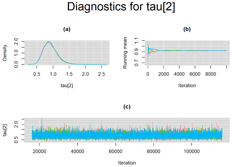
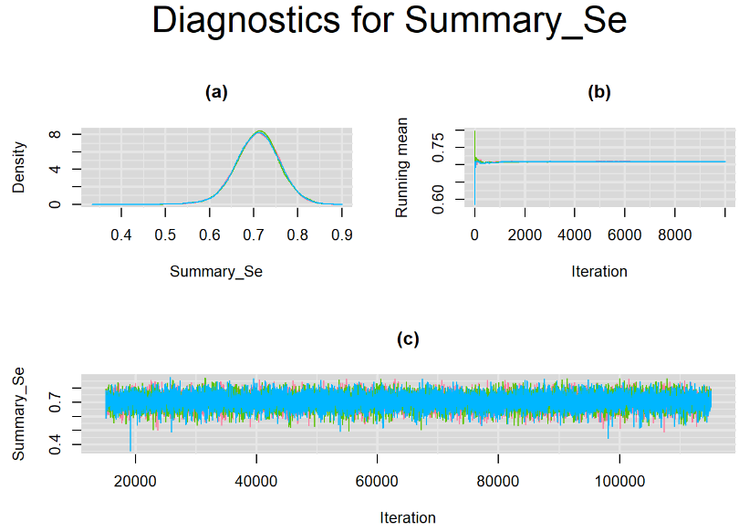
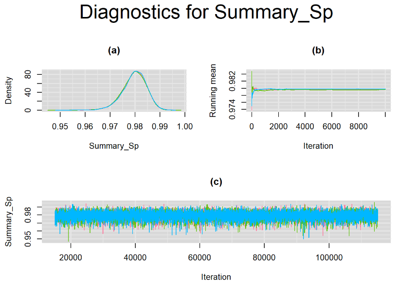
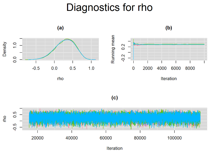
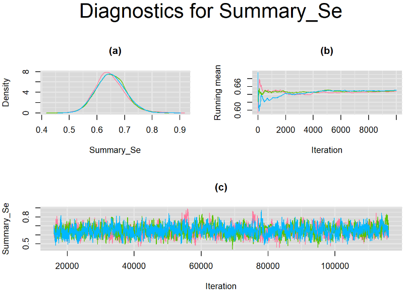
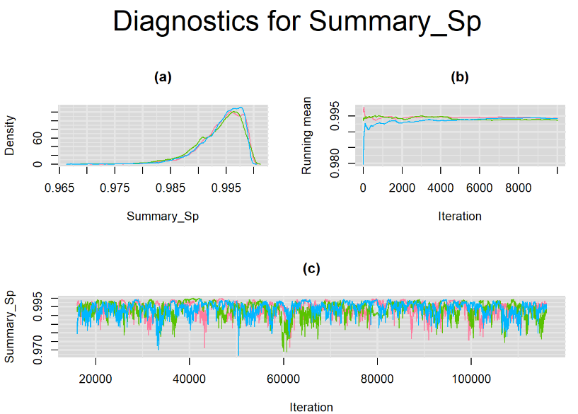
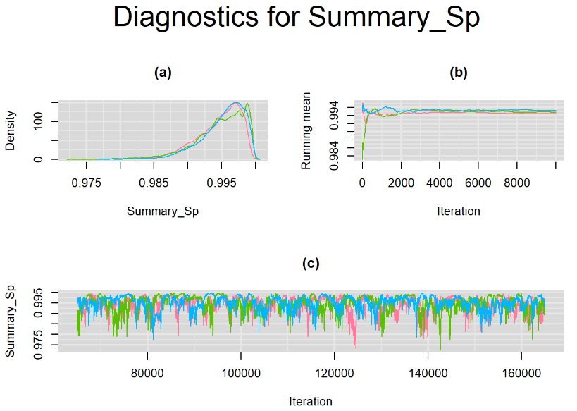
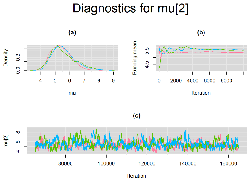
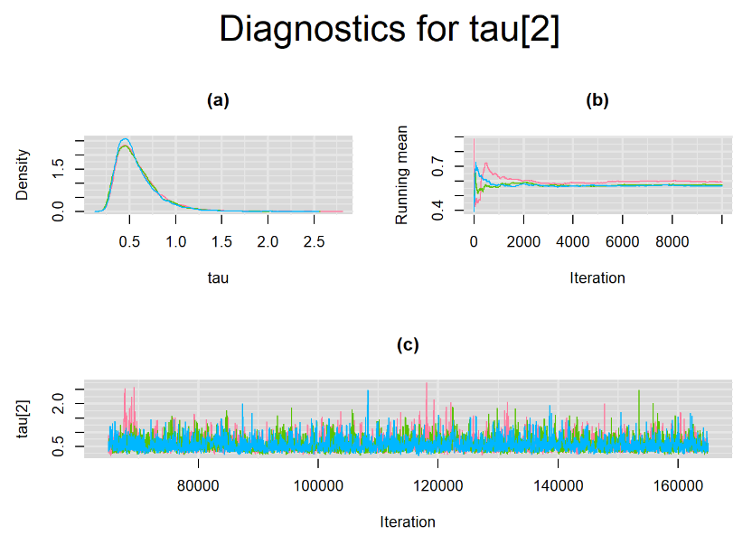
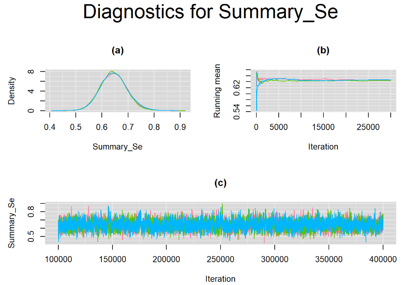
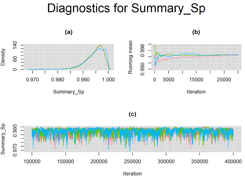
datatable(output_LC_1000, extensions = 'AutoFill', options = list(autoFill = TRUE))According to our bivariate latent class model, when culture test is imperfect, the mean sensitivity (Summary_Se) and mean specificity (Summary_Sp) of Xpert are estimated to be 64.73% [95% credible interval : 55.03 - 76] and 99.49% [95% credible interval : 98.44 - 99.91], respectively. The Gelman-Rubin statistics for both parameters are Rhat= 1 and Rhat= 1.05, respectively. As for their effective sample size, n.eff= 745 and n.eff= 332, respectively. They could be seen to be a bit low. For instance, this would mean that despite that our posterior sample for Summary_Sp is based on 30,000 iterations, the posterior estimate of 99.49% would correspond to an estimate obtained from a simple random sampling of only 332 only.
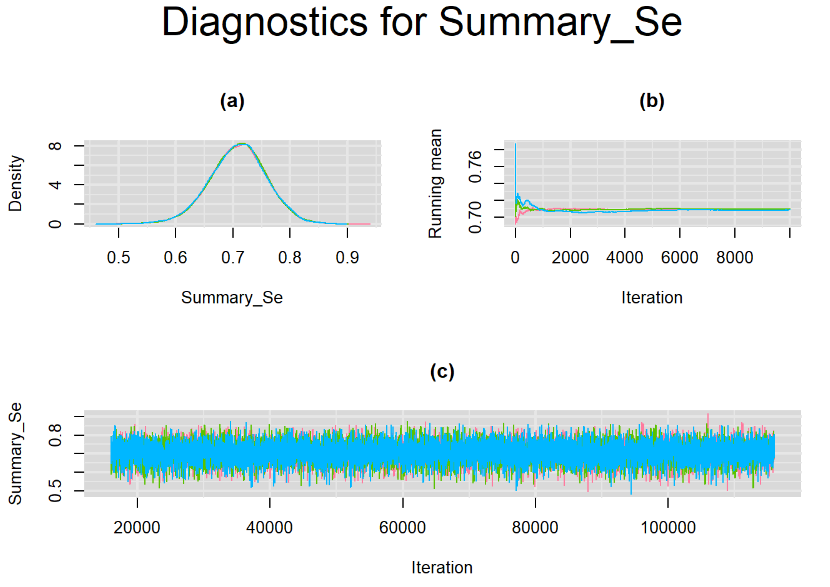
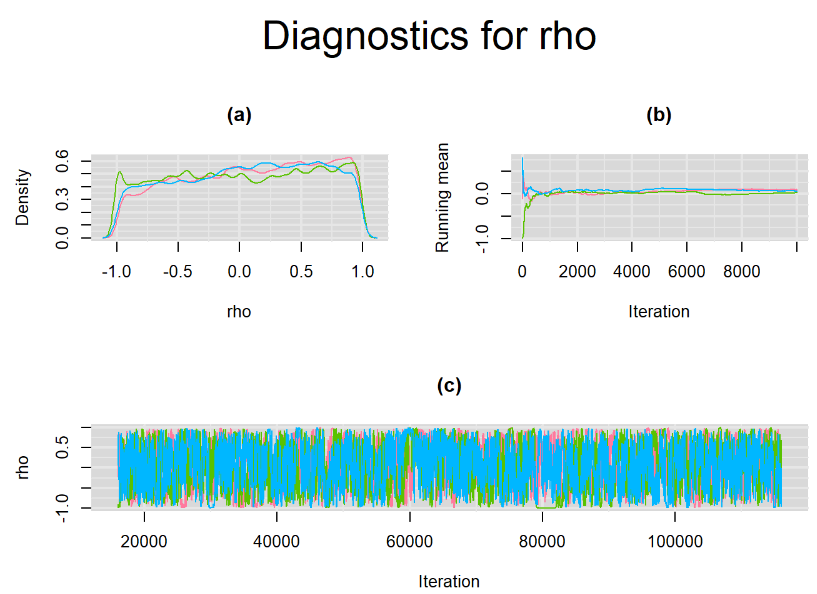
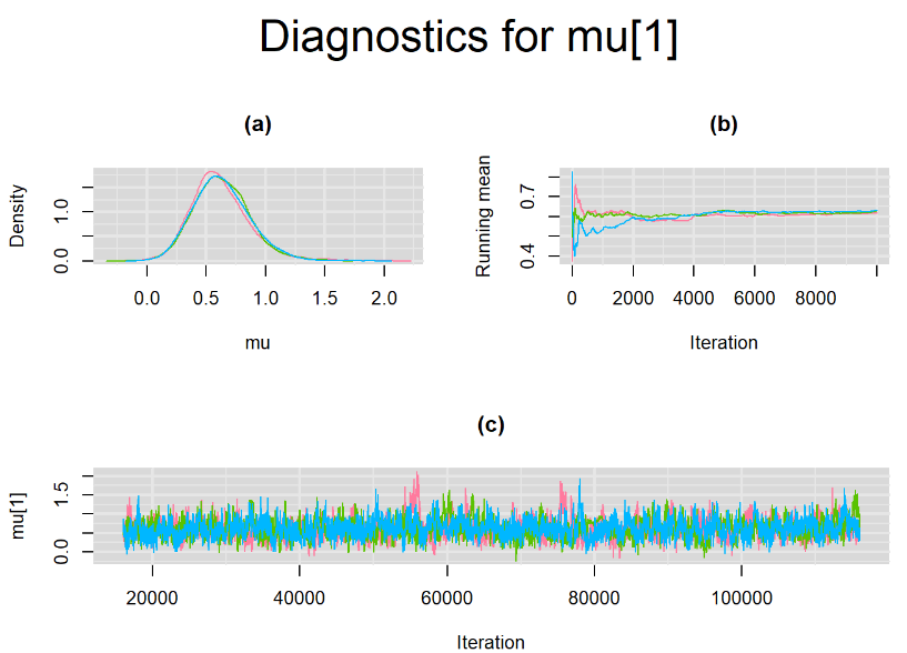
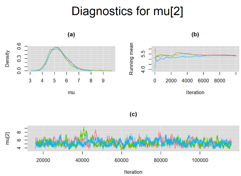
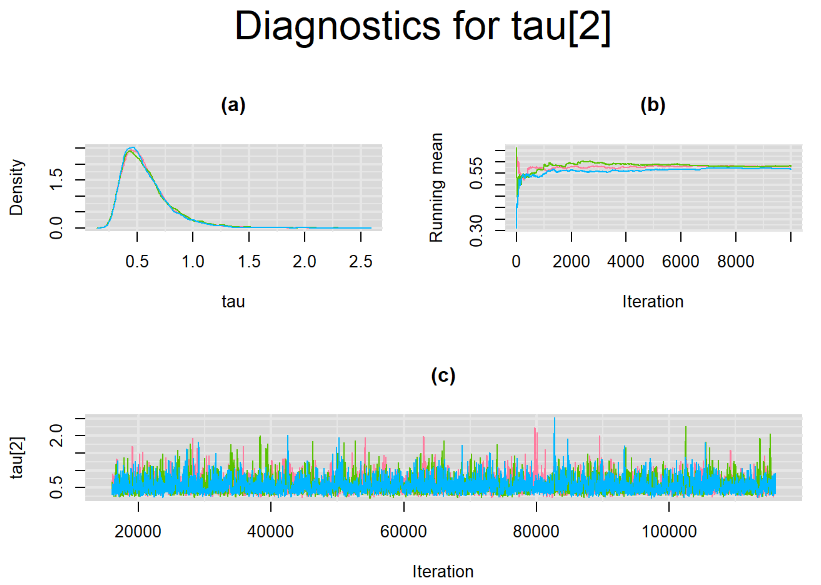
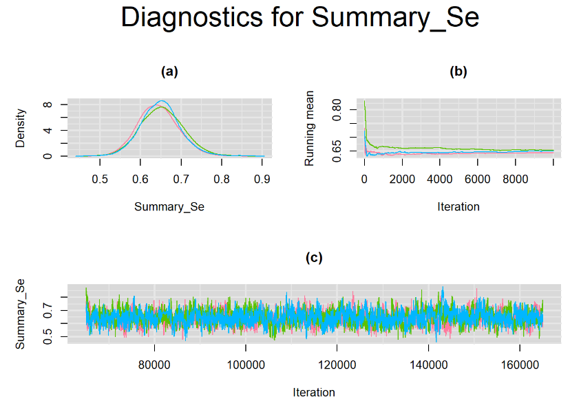
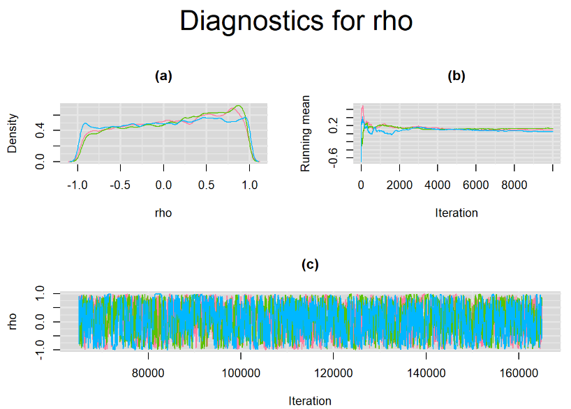
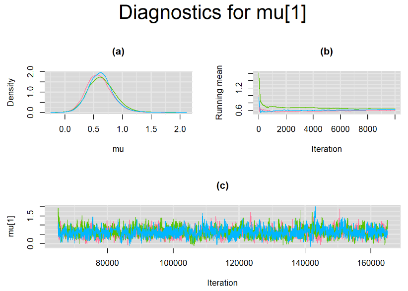
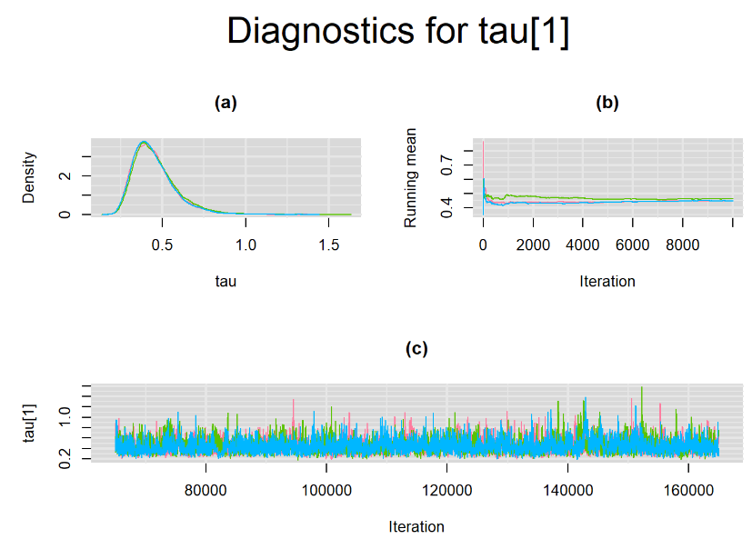
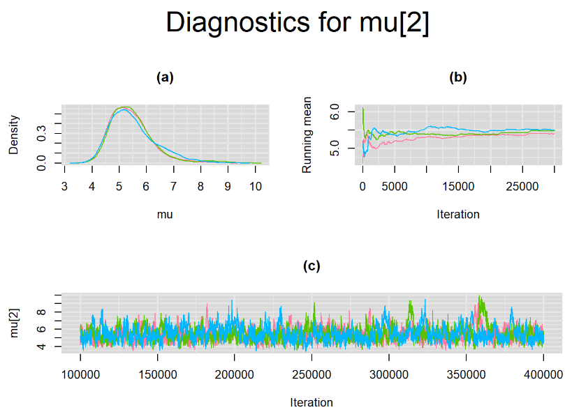
Browsing the results we can see that the Gelman-Rubin statistics differs from 1 for a non negligible amount of parameters. Below are convergence plots for a subset of the parameters. A look at the density, trace and running mean plots shows that all 3 chains are converging to solutions that are close to each other. For some parameters, like Summary_Sp, the density curves might not look as smooth as we would wish for. Is this a problem with the adaptation phase failing to complete or could we improve by increasing the number of iterations?
SETTINGS NUMBER 2
Before increasing the number of iterations, we followed the JAGS manual recommendation, i.e. we decided to re-run the model from scratch by increasing the n.adapt argument of the jags.model function from 1000 to 50000 adaptive iterations, hoping that this would be enough to complete the adaptation phase in order to bring the sampler to an optimal sampling behavior, and possibly improve parameter convergence. Our setttings were therefore as followed
- 3-chain model
- Adaptation phase of
50000iterations - Burn-in phase of
15000iterations - Draw
100000more iterations with a thinning value of 10 to estimate the posterior distribution of each parameter with a posterior sample of10000iterations for each chain resulting in a final posterior sample of30000iterations for each parameter.
# Compile the model
jagsModel = jags.model("model.txt",data=dataList,n.chains=3,inits=initsList,n.adapt=50000)
Despite running 50000 iterations during the adaptation phase, it was still apparently not enough to allow the sampler to tune up its own parameters to behave optimally. Once more, this did not prevent us from obtaining posterior samples from which we calculated the following posterior estimates
# Summary statistics
output_LC_50000 <- read.table("output_LC_50000.txt",header=TRUE)
colnames(output_LC_50000)[4:6] <- c("2.5%", "50%", "97.5%")
datatable(output_LC_50000, extensions = 'AutoFill', options = list(autoFill = TRUE))
The mean sensitivity (Summary_Se) and mean specificity (Summary_Sp) estimates of Xpert were not much different than the ones obtained with n.adapt = 1,000. This time, Summary_Se = 64.71% [95% credible interval : 55.29 - 75.1] while Summary_Sp = 99.55% [95% credible interval : 98.64 - 99.93]. The Gelman-Rubin statistics for both parameters are Rhat= 1 and Rhat= 1.01, respectively. Their effective sample size are also similar to the case when the adaptation step counts 1000 iterations, n.eff= 944 and n.eff= 322, respectively.
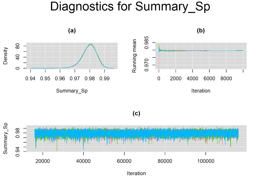
Their respective density, history and running mean plots are also behaving quite similarly to the ones when n.adapt = 1,000 as seen below.
SETTINGS NUMBER 3
We did not achieve an optimal sampler despite running 50000 adaptive iterations and it did not seem to improve convergence. If JAGS’ sampler cannot achieve optimal behavior, then could we run more burn-in and sampling iterations to compensate ?
With that in mind, we ran a 3-chain model with the following specifications :
- Adaptation phase of
50000iterations - Burn-in phase of
50000iterations - Draw
300000more iterations with a thinning value of 10 to estimate the posterior distribution of each parameter with a posterior sample of30000iterations for each chain
This resulted in a final posterior sample of 90000 iterations for each parameter.

Once more the Adaptation incomplete warning was triggered. Posterior estimates were as followed
# Summary statistics
output_LC_50000_large_burn <- read.table("output_LC_50000_large_burn.txt",header=TRUE)
colnames(output_LC_50000_large_burn)[4:6] <- c("2.5%", "50%", "97.5%")
datatable(output_LC_50000_large_burn, extensions = 'AutoFill', options = list(autoFill = TRUE))
The mean sensitivity (Summary_Se) and mean specificity (Summary_Sp) estimates of Xpert were once more very similar to the ones obtained with both n.adapt = 1,000 and n.adapt = 50,000, with Summary_Se = 64.35% [95% credible interval : 54.73 - 74.81] while Summary_Sp = 99.52% [95% credible interval : 98.57 - 99.94]. The Gelman-Rubin statistics for both parameters are Rhat= 1 and Rhat= 1, respectively. Their effective sample size are larger with n.eff= 2307 and n.eff= 854, respectively, but they are proportionally similar with respect to their total posterior samples.
Increasing the number of burn-in and sampling iterations had a beneficial impact on convergence, i.e. smooting the density curves and lowering almost every parameter’s Gelman-Ruben statistics to 1.
SETTINGS NUMBER 4
Taking advantage of prior knowledge on culture test for TB meningitis, we decided to inject some informative prior in the model of settings number 3. Since it is believed that the culture (reference) test has a near perfect specificity, we incorporate this information in our model by specifying an informative prior distribution for the parameter mu2[2]. A normal distribution with mean=4 and precision=4 is placed on mu2[2]. This prior distribution places much of its weight on probability values that are greater than 0.95
# Compile the model
jagsModel = jags.model("model_inform_prior.txt",data=dataList,n.chains=3,inits=initsList,n.adapt=50000)
Once more the Adaptation incomplete warning was triggered.
 Posterior estimates were as followed
# Summary statistics
output_LC_50000_large_burn_inform <- read.table("output_LC_50000_large_burn_inform.txt",header=TRUE)
colnames(output_LC_50000_large_burn_inform)[4:6] <- c("2.5%", "50%", "97.5%")
datatable(output_LC_50000_large_burn_inform, extensions = 'AutoFill', options = list(autoFill = TRUE))
The mean sensitivity (Summary_Se) and mean specificity (Summary_Sp) estimates of Xpert were once more very similar to the ones obtained in previous settings with Summary_Se = % [95% credible interval : - ] while Summary_Sp = % [95% credible interval : - ]. The Gelman-Rubin statistics for both parameters are Rhat= and Rhat= , respectively. Their effective sample size are larger with n.eff= and n.eff= , respectively, but they are proportionally similar with respect to their total posterior samples.
Results were remarkably similar among all 4 settings described in the previous sections above. Despite the warning triggered for all 4 settings studied, the consistency in the posterior estimates gives us some confidence in the results. To get even more certainty in those posterior estimates, we will try to validate one more time with a different software …
BIVARIATE LATENT CLASS MODEL WITH OpenBUGS
From our previous attempts at running the model, it’s clear that our changes did not have a big impact on the posterior parameter estimates. However, all attempts triggered the Adaptation incomplete warning. So, is it a bad thing? To try to answer that question, we are going to run the same bivariate latent class model on the same data using OpenBUGS software. This software is the open source program for Bayesian analysis using MCMC sampling that was developed from WinBUGS ((Lunn et al(2000))).
In OpenBUGS, the model, the data as well as the initial values must be first defined in separate files (i.e. txt files) before being read in the software. Below we are only reporting the posterior estimates obtained in OpenBUGS for the latent class meta-analysis model. For the initial values, we selected them to match the ones that were generated in our rjags bivariate latent class examples above. For the interested reader, all the files and script will be available in one of the link at the end of this blog article.
The mean sensitivity (Summary_Se) and mean specificity (Summary_Sp) estimates of Xpert were once more very similar to the ones obtained with rjags pacakge, with Summary_Se = 63.86% [95% credible interval : 54.4 - 74.05] while Summary_Sp = 99.67% [95% credible interval : 98.68 - 99.97].
When running a model in OpenBUGS software, the adapting box will be ticked while the MCMC algorithm is in its adaptive phase as seen below.
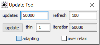
Once the initial tuning of the adaptation phase is completed, the adapting box is no longer ticked as seen below from the model we obtained the posterior results displayed in this section. We believe this is suggesting that the simulation did complete its adaptation phase.
CONCLUSION
In this blog article we looked at the possible impact on the posterior samples of a sampler not behaving optimally. This question arose because in some instances, the jags.model function will return a Adaptation incomplete warning. We found no difference, aside from random sampling errors, between a bivariate model with a sampler fully optimized and the same model with a sampler behaving sup-optimally. In the case of the more complex bivariate latent class model which seems to constantly trigger the warning, varying the number of adaptive, burn-in and sampling iterations as well as providing prior information or using a different software did not have an impact on the posterior estimates which remained consistent across all settings. The convergence statistics, such as the Gelman-Rubin statistics as well as trace plots did not show any lack of convergence, especially with large sampling iterations, giving us faith in the posterior estimates. Our conclusions would therefore be that the warning can probably be ignored especially if a large number of sampling iterations is run resulting in satisfying convergence behavior of the parameters.
REFERENCES
Citation
@online{schiller2021,
  author = {Ian Schiller and Nandini Dendukuri},
  title = {A Journey into the Adaptive Phase of an {MCMC} Algorithm},
  date = {2021-06-21},
  url = {https://www.nandinidendukuri.com/blogposts/2021-06-21-adaptation_incomplete/},
  langid = {en}
}