library(rjags)
library(mcmcplots)Here are some examples of fitting simple statistical models in rjags. They are useful for beginners learning Bayesian inference using the rjags library. Notice in each case all that is required is specification of the probability density function for the observed data (i.e. the likelihood function) and the prior distribution functions for the unknown parameters.
Beyond that the user needs to be familiar with the rjags syntax for compiling the model, running the MCMC algorithm, sampling from the posterior distribution and examining the sample. The mcmcplots library is necessary for the last step.
These example programs were first written in WinBUGS by Lawrence Joseph. They were reprogrammed using R Markdown by Mandy Yao.
Loading the necessary libraries
Binomial Proportion
modelString =
  "model {

    x~dbin(theta,n)        #  Likelihood function

    theta ~ dbeta(1,1)     #  Prior density for theta

  }"

#Write the model to a file
writeLines(modelString,con="model.txt")

#Compiling the model together with the data
jagsModel = jags.model("model.txt",data=list(x=6,n=20))
Compiling model graph
Resolving undeclared variables
Allocating nodes
Graph information:
Observed stochastic nodes: 1
Unobserved stochastic nodes: 1
Total graph size: 4
Initializing model#Burn-in
update(jagsModel,n.iter=5000)
# The parameter(s) to be monitored.
parameters = c( "theta")
#Sampling from the posterior distribution:
output = coda.samples(jagsModel,variable.names=parameters,n.iter=10000)
# Examining the posterior sample
# Density plots
denplot(output, parms=c("theta"))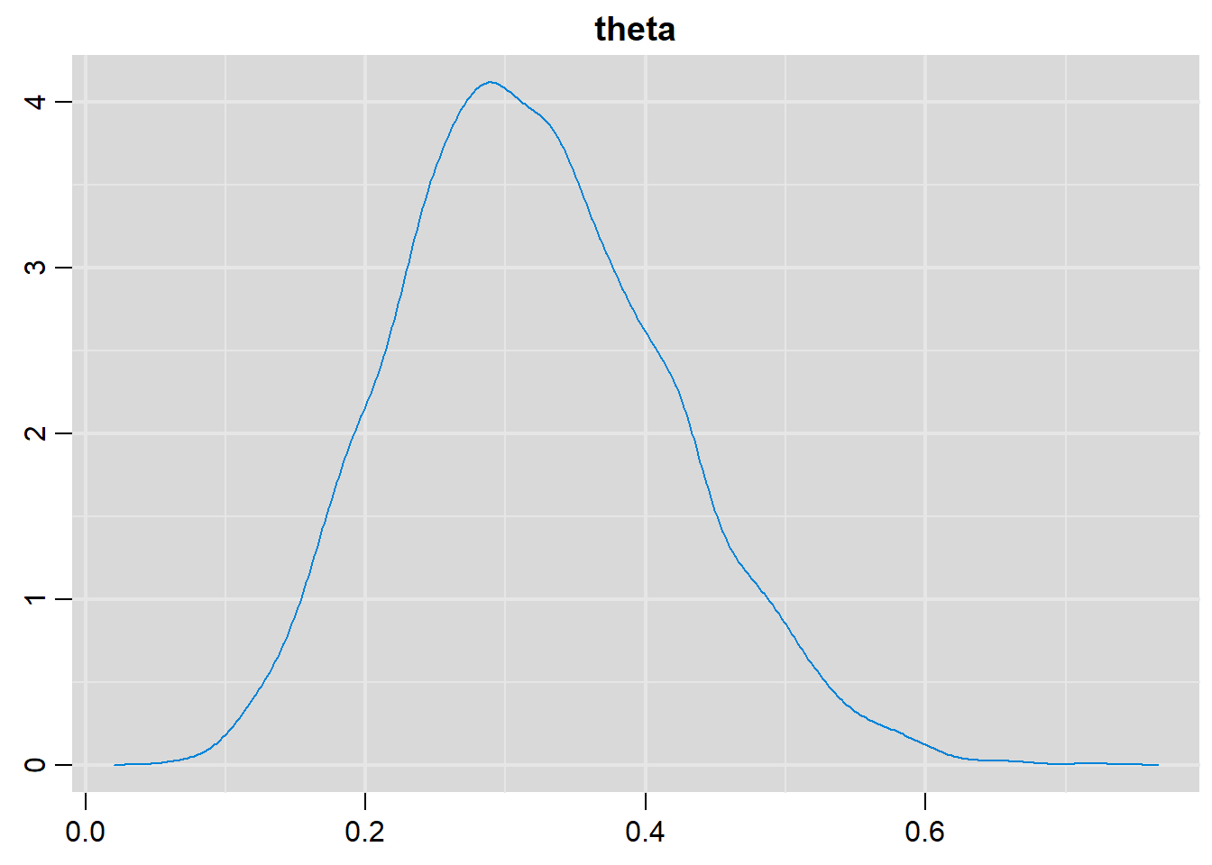
# History plot(s)
traplot(output, parms=c("theta"))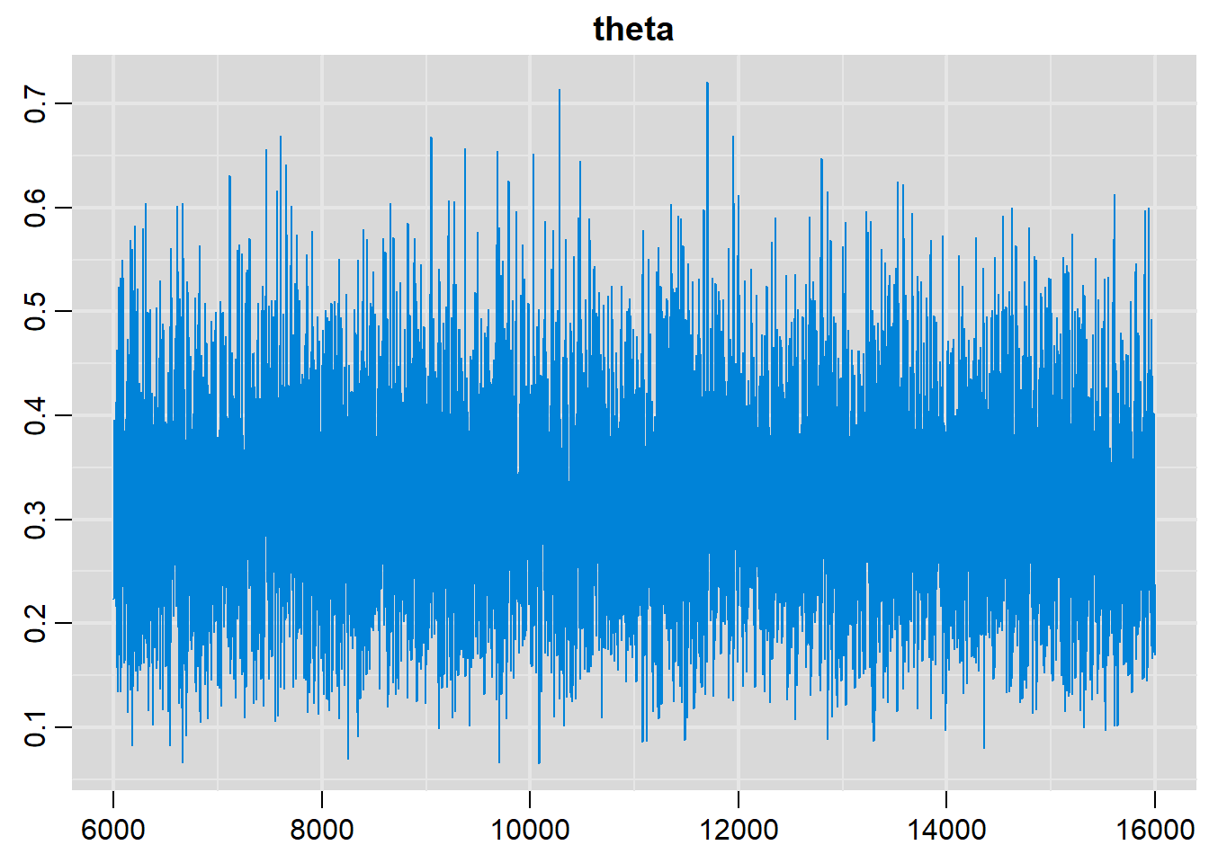
# Summary statistics
summary(output)
Iterations = 6001:16000
Thinning interval = 1
Number of chains = 1
Sample size per chain = 10000

1. Empirical mean and standard deviation for each variable,
   plus standard error of the mean:

          Mean             SD       Naive SE Time-series SE
      0.319664       0.096402       0.000964       0.001303

2. Quantiles for each variable:

  2.5%    25%    50%    75%  97.5%
0.1501 0.2508 0.3129 0.3835 0.5225
Binomial Proportion Difference
modelString =
  "model { x  ~ dbin(theta1, n1)   #  Likelihood for group 1
         theta1 ~ dbeta(1,1)         #  Prior for theta1

         y  ~ dbin(theta2, n2)   #  Likelihood for group 2
         theta2 ~ dbeta(1,1)         #  Prior for theta2

      propdiff <- theta1-theta2        #  Calculate difference for binomial parameters
      rr <- theta1/theta2              #  Calculate relative risk
                                       #  Calculate odds ratio
      or<- theta1*(1-theta2)/((1-theta1)*theta2)
  }"

#Write the model to a file
writeLines(modelString,con="model.txt")

#Compiling the model together with the data
jagsModel = jags.model("model.txt",data=list(x  = 6,
                                             n1 = 20,
                                             y  = 20,
                                             n2 = 25))
Compiling model graph
Resolving undeclared variables
Allocating nodes
Graph information:
Observed stochastic nodes: 2
Unobserved stochastic nodes: 2
Total graph size: 14
Initializing model#Burn-in
update( jagsModel,n.iter=5000)
# The parameter(s) to be monitored.
parameters = c( "theta1", "theta2", "propdiff", "or", "rr")
#Sampling from the posterior distribution:
output = coda.samples(jagsModel,variable.names=parameters,n.iter=10000)
# Examining the posterior sample
# History plots
traplot(output, parms=c("propdiff"))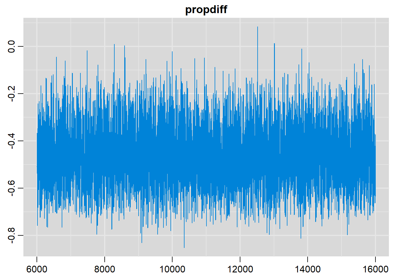
# Density plots
denplot(output, parms=c("propdiff"))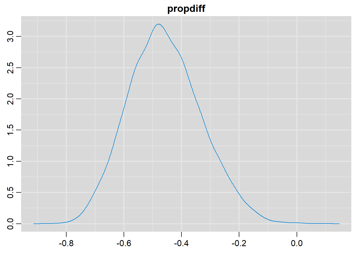
# Summary statistics
summary(output)
Iterations = 6001:16000
Thinning interval = 1
Number of chains = 1
Sample size per chain = 10000

1. Empirical mean and standard deviation for each variable,
   plus standard error of the mean:

            Mean      SD  Naive SE Time-series SE
or        0.1510 0.10721 0.0010721       0.001449
propdiff -0.4581 0.12547 0.0012547       0.001651
rr        0.4161 0.13543 0.0013543       0.001753
theta1    0.3204 0.09771 0.0009771       0.001249
theta2    0.7785 0.07869 0.0007869       0.001036

2. Quantiles for each variable:

             2.5%      25%     50%     75%   97.5%
or        0.03042  0.07758  0.1230  0.1924  0.4294
propdiff -0.68789 -0.54732 -0.4643 -0.3759 -0.2005
rr        0.18627  0.31835  0.4054  0.5010  0.7093
theta1    0.14726  0.24917  0.3144  0.3850  0.5246
theta2    0.60620  0.72813  0.7855  0.8362  0.9109
Normal Mean, Known Variance
modelString =
  "model { for (i in 1:n)
      {
         x[i]   ~   dnorm(mu,tau)    #  Likelihood function for each data point
       }
         mu     ~   dnorm(0,0.0001)  #  Prior for mu
         tau    <- 1                 #  Prior for tau, actually a fixed value
         sigma  <-  1/sqrt(tau)      #  Prior for sigma (as a function of tau)
  }"

#Write the model to a file
writeLines(modelString,con="model.txt")

#Compiling the model together with the data
jagsModel = jags.model("model.txt",data=list(x=c(-1.10635822,  0.56352639, -1.62101846,  0.06205707,  0.50183464,
0.45905694, -1.00045360, -0.58795638,  1.01602187, -0.26987089, 0.18354493 , 1.64605637, -0.96384666,  0.53842310, -1.11685831, 0.75908479 , 1.10442473 , -1.71124673, -0.42677894 , 0.68031412), n=20))
Compiling model graph
Resolving undeclared variables
Allocating nodes
Graph information:
Observed stochastic nodes: 20
Unobserved stochastic nodes: 1
Total graph size: 27
Initializing model#Burn-in
update( jagsModel,n.iter=5000)
# The parameter(s) to be monitored.
parameters = c( "mu")
#Sampling from the posterior distribution
output = coda.samples(jagsModel,variable.names=parameters,n.iter=10000)
# Examining the posterior sample
# History plots
traplot(output, parms=c("mu"))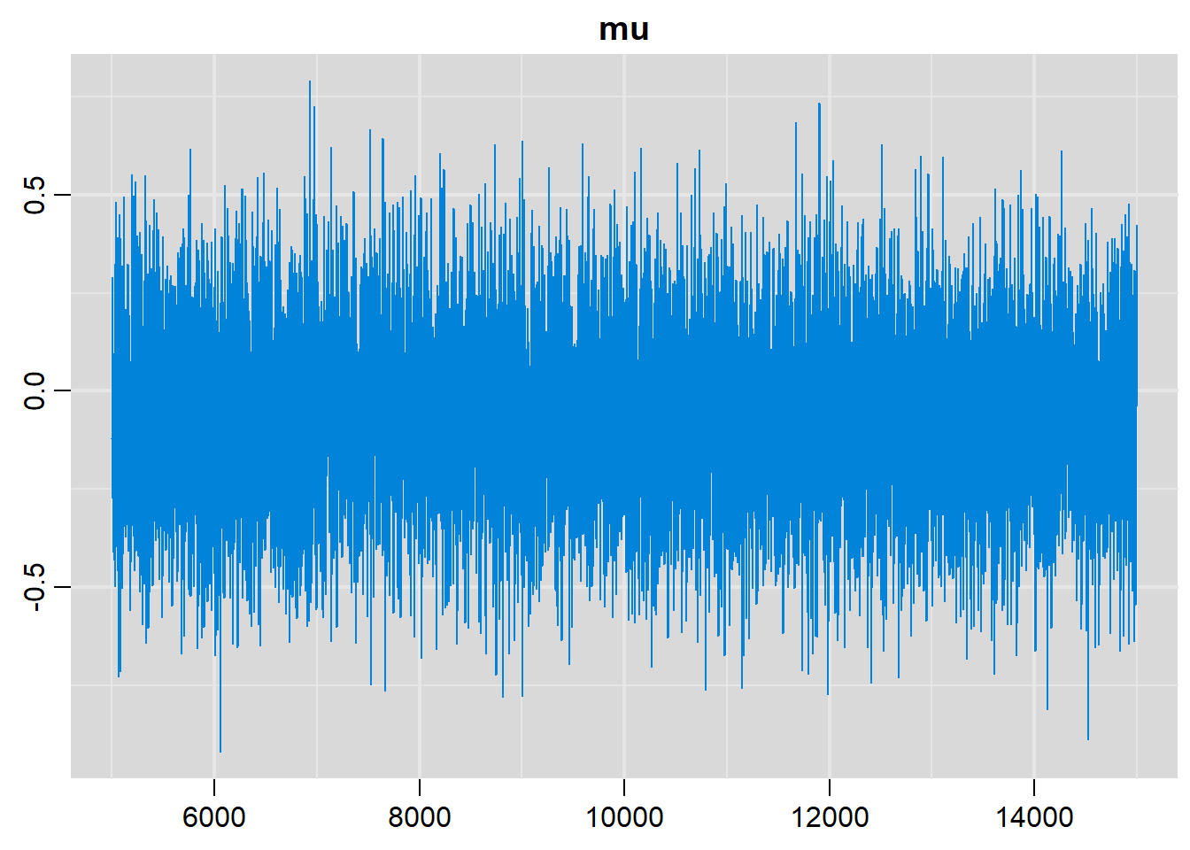
# Density plots
denplot(output, parms=c("mu"))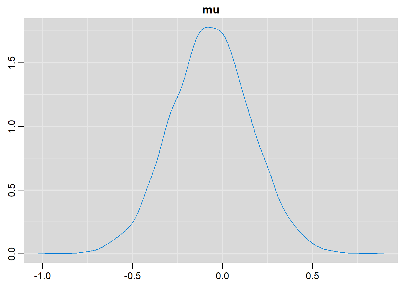
# Summary statistics
summary(output)
Iterations = 5001:15000
Thinning interval = 1
Number of chains = 1
Sample size per chain = 10000

1. Empirical mean and standard deviation for each variable,
   plus standard error of the mean:

          Mean             SD       Naive SE Time-series SE
     -0.063596       0.222696       0.002227       0.002227

2. Quantiles for each variable:

    2.5%      25%      50%      75%    97.5%
-0.50055 -0.21340 -0.06442  0.08385  0.37717
Normal Mean, Unknown Variance
modelString =
  "model { for (i in 1:n)
      {
         x[i]   ~  dnorm(mu,tau)     #  Likelihood function for each data point
       }
         mu     ~  dnorm(0,0.0001)   #  Prior for mu
         tau    <- 1/(sigma*sigma)   #  Prior for tau (as function of sigma)
         sigma  ~  dunif(0,20)       #  Prior for sigma
  }"

#Write the model to a file
writeLines(modelString,con="model.txt")

#Compiling the model together with the data
jagsModel = jags.model("model.txt",data=list(x=c( -1.10635822,  0.56352639, -1.62101846,  0.06205707,  0.50183464, 0.45905694,  -1.00045360, -0.58795638,  1.01602187, -0.26987089 , 0.18354493 , 1.64605637, -0.96384666,  0.53842310, -1.11685831, 0.75908479 , 1.10442473 , -1.71124673,  -0.42677894 , 0.68031412), n=20), inits = list(mu=1, sigma=1))
Compiling model graph
Resolving undeclared variables
Allocating nodes
Graph information:
Observed stochastic nodes: 20
Unobserved stochastic nodes: 2
Total graph size: 29
Initializing model#Burn-in
update( jagsModel,n.iter=5000)
# The parameter(s) to be monitored.
parameters = c("mu", "sigma", "tau")
#Sampling from the posterior distribution
output = coda.samples(jagsModel,variable.names=parameters,n.iter=10000)
# Examining the posterior sample
# History plots
traplot(output, parms=c("mu", "tau"))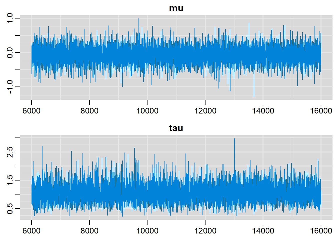
# Density plots
denplot(output, parms=c("mu", "tau"))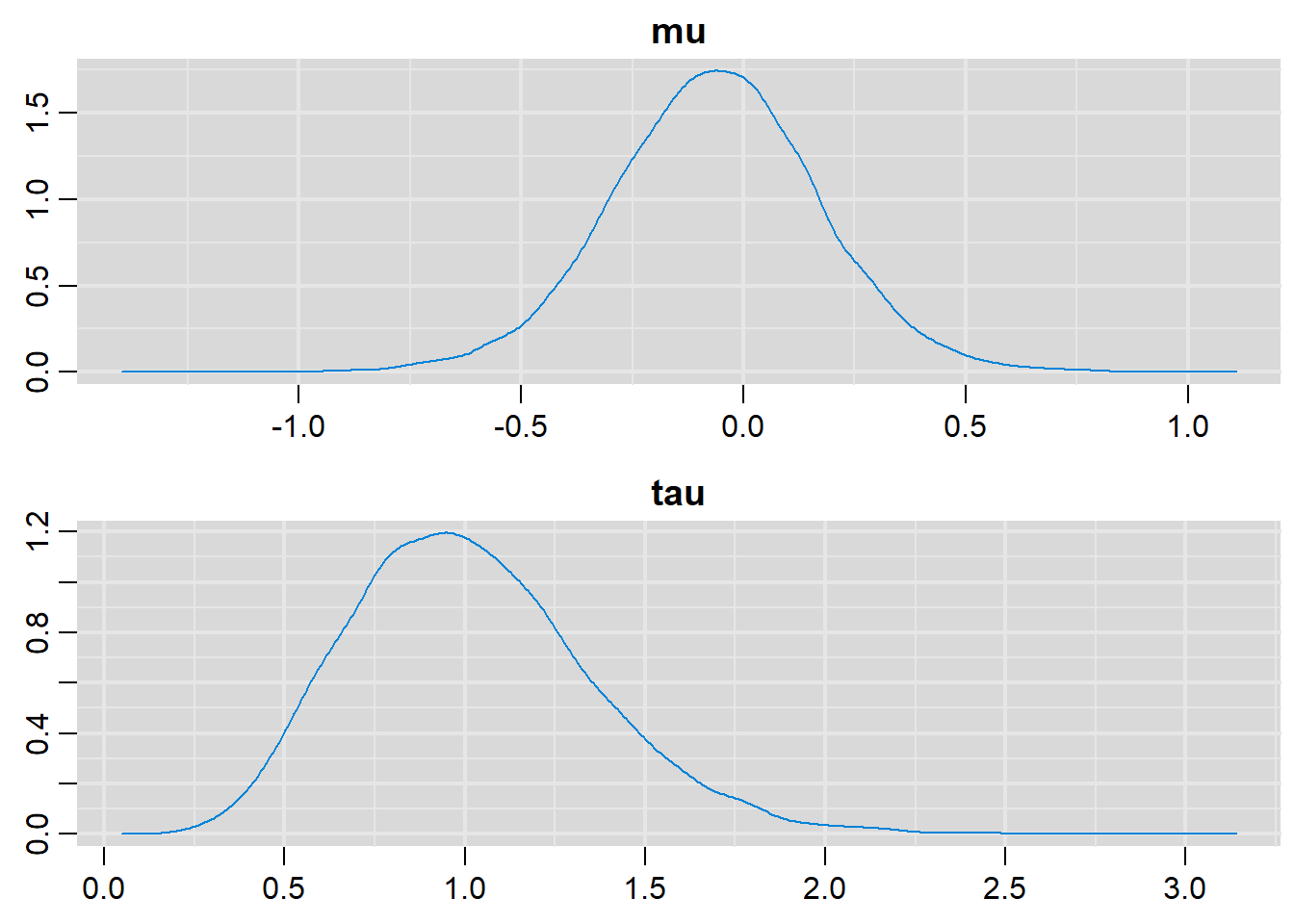
# Summary statistics
summary(output)
Iterations = 6001:16000
Thinning interval = 1
Number of chains = 1
Sample size per chain = 10000

1. Empirical mean and standard deviation for each variable,
   plus standard error of the mean:

          Mean     SD Naive SE Time-series SE
mu    -0.06476 0.2360 0.002360       0.002318
sigma  1.03540 0.1873 0.001873       0.002898
tau    1.01759 0.3352 0.003352       0.004732

2. Quantiles for each variable:

         2.5%     25%      50%    75%  97.5%
mu    -0.5411 -0.2178 -0.06336 0.0876 0.4029
sigma  0.7549  0.9044  1.00545 1.1344 1.4838
tau    0.4542  0.7771  0.98920 1.2226 1.7550
Linear Regression
modelString =
  "model { for (i in 1:n) {
     mu[i]  <- alpha + b.sex*sex[i] + b.age*age[i]   # Regression function

     bp[i]   ~ dnorm(mu[i],tau)                      # Normal likelihood terms for each data point

    }
    alpha    ~ dnorm(0.0,1.0E-4)
    b.sex    ~ dnorm(0.0,1.0E-4)
    b.age    ~ dnorm(0.0,1.0E-4)
    tau     <-  1/(sigma*sigma)                      # Prior for tau as function of sigma
    sigma    ~  dunif(0,20)                          # Prior directly on sigma
  }"

#Write the model to a file
writeLines(modelString,con="model.txt")


#Compiling the model together with the data
jagsModel = jags.model("model.txt",data=list(
  sex = c(0, 1, 0, 0, 0, 1, 0, 1, 1, 0, 1, 0, 0, 0, 0, 1, 0, 1, 0, 0,
          1, 0, 1, 0, 0, 0, 1, 1, 1, 1),
  age = c(59, 52, 37, 40, 67, 43, 61, 34, 51, 58, 54, 31, 49, 45, 66, 48, 41, 47, 53, 62,
          60, 33, 44, 70, 56, 69, 35, 36, 68, 38),
  bp = c(143, 132, 88, 98, 177, 102, 154, 83, 131, 150, 131, 69, 111, 114, 170, 117, 96, 116, 131, 158,
         156, 75, 111, 184, 141, 182, 74, 87, 183, 89),
  n=30), list(alpha=50, b.sex=1, b.age=4))
Compiling model graph
Resolving undeclared variables
Allocating nodes
Graph information:
Observed stochastic nodes: 30
Unobserved stochastic nodes: 4
Total graph size: 163
Initializing model#Burn-in
update( jagsModel,n.iter=5000)
# The parameter(s) to be monitored.
parameters = c("mu", "alpha", "b.age", "b.sex", "tau", "sigma")
#Sampling from the posterior distribution:
output = coda.samples(jagsModel,variable.names=parameters,n.iter=10000)
# Examining the posterior sample
# History plots
traplot(output, parms=c("alpha", "b.age", "b.sex", "tau"))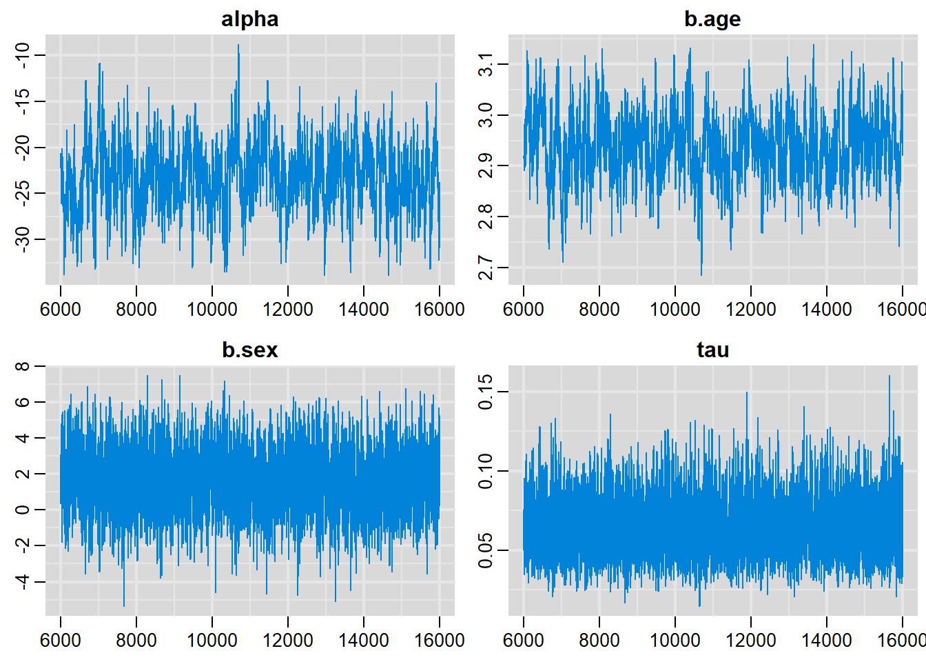
# Density plots
denplot(output, parms=c("alpha", "b.age", "b.sex", "tau"))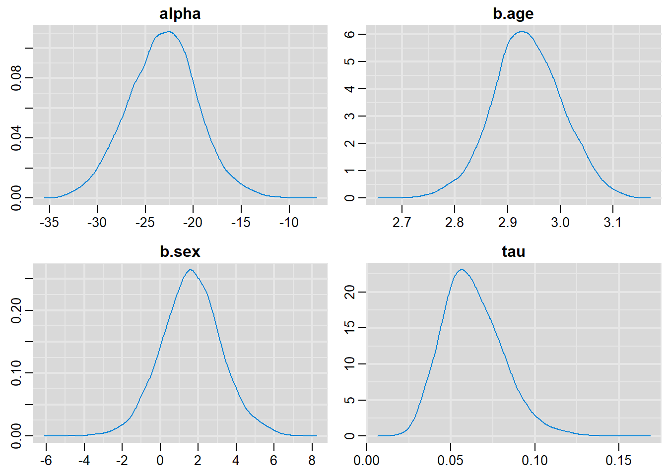
# Summary statistics
summary(output)
Iterations = 6001:16000
Thinning interval = 1
Number of chains = 1
Sample size per chain = 10000

1. Empirical mean and standard deviation for each variable,
   plus standard error of the mean:

            Mean      SD  Naive SE Time-series SE
alpha  -23.17305 3.59794 0.0359794      0.2247397
b.age    2.93765 0.06542 0.0006542      0.0039830
b.sex    1.63572 1.58828 0.0158828      0.0350342
mu[1]  150.14824 1.07578 0.0107578      0.0189276
mu[2]  131.22042 1.21586 0.0121586      0.0205117
mu[3]   85.51996 1.43855 0.0143855      0.0699601
mu[4]   94.33291 1.30427 0.0130427      0.0616028
mu[5]  173.64943 1.36112 0.0136112      0.0496858
mu[6]  104.78158 1.20244 0.0120244      0.0183570
mu[7]  156.02354 1.13128 0.0113128      0.0253913
mu[8]   78.34274 1.45143 0.0145143      0.0541390
mu[9]  128.28277 1.20020 0.0120020      0.0184350
mu[10] 147.21059 1.05304 0.0105304      0.0148822
mu[11] 137.09572 1.25685 0.0125685      0.0292534
mu[12]  67.89407 1.74273 0.0174273      0.0952851
mu[13] 120.77175 1.02878 0.0102878      0.0259468
mu[14] 109.02115 1.12181 0.0112181      0.0421145
mu[15] 170.71178 1.31749 0.0131749      0.0454469
mu[16] 119.46982 1.17401 0.0117401      0.0153321
mu[17]  97.27056 1.26312 0.0126312      0.0574121
mu[18] 116.53218 1.17248 0.0117248      0.0150763
mu[19] 132.52235 0.99762 0.0099762      0.0137313
mu[20] 158.96119 1.16356 0.0116356      0.0291061
mu[21] 154.72161 1.44539 0.0144539      0.0498572
mu[22]  73.76937 1.63717 0.0163717      0.0873575
mu[23] 107.71923 1.18963 0.0118963      0.0162000
mu[24] 182.46238 1.50154 0.0150154      0.0624519
mu[25] 141.33529 1.01870 0.0101870      0.0130165
mu[26] 179.52473 1.45330 0.0145330      0.0581969
mu[27]  81.28039 1.41386 0.0141386      0.0498558
mu[28]  84.21804 1.37837 0.0137837      0.0456021
mu[29] 178.22280 1.80215 0.0180215      0.0840347
mu[30]  90.09333 1.31430 0.0131430      0.0372826
sigma    4.11184 0.61440 0.0061440      0.0109576
tau      0.06295 0.01787 0.0001787      0.0002809

2. Quantiles for each variable:

            2.5%       25%       50%       75%    97.5%
alpha  -30.24650 -25.62284 -23.09952 -20.79735 -15.9642
b.age    2.80601   2.89440   2.93620   2.98143   3.0664
b.sex   -1.48859   0.60841   1.63069   2.65494   4.8785
mu[1]  147.98904 149.43674 150.13293 150.87232 152.2680
mu[2]  128.83427 130.40717 131.22674 132.03090 133.6199
mu[3]   82.65874  84.56967  85.52605  86.46476  88.3713
mu[4]   91.74115  93.48355  94.33728  95.19132  96.9032
mu[5]  170.95790 172.73937 173.64600 174.55836 176.3252
mu[6]  102.39861 103.98984 104.78427 105.57633 107.1499
mu[7]  153.76994 155.27964 156.00774 156.78553 158.2422
mu[8]   75.44941  77.38705  78.34408  79.29536  81.2263
mu[9]  125.94022 127.47654 128.28494 129.07648 130.6641
mu[10] 145.09643 146.51176 147.19439 147.92167 149.2635
mu[11] 134.63377 136.24648 137.10151 137.92964 139.6156
mu[12]  64.42218  66.73557  67.90819  69.03915  71.3939
mu[13] 118.75822 120.10111 120.76888 121.44737 122.7899
mu[14] 106.81223 108.28542 109.01908 109.75978 111.2136
mu[15] 168.10918 169.83039 170.70258 171.59128 173.3127
mu[16] 117.18030 118.68070 119.47295 120.24638 121.7831
mu[17]  94.77249  96.44715  97.27374  98.10866  99.7510
mu[18] 114.22169 115.74728 116.53277 117.31122 118.8344
mu[19] 130.54712 131.86596 132.51227 133.19156 134.4915
mu[20] 156.63397 158.19683 158.95159 159.74785 161.2494
mu[21] 151.85451 153.75361 154.71497 155.66527 157.6127
mu[22]  70.51600  72.68436  73.78254  74.84522  77.0423
mu[23] 105.35989 106.94205 107.72874 108.50281 110.0698
mu[24] 179.50180 181.44971 182.45246 183.46765 185.4481
mu[25] 139.29631 140.66017 141.32104 142.01697 143.3280
mu[26] 176.66255 178.54980 179.51723 180.50334 182.4096
mu[27]  78.46788  80.35473  81.28410  82.21174  84.0738
mu[28]  81.48508  83.31126  84.22462  85.11676  86.9264
mu[29] 174.67538 177.03429 178.22617 179.41572 181.7924
mu[30]  87.48664  89.23480  90.10345  90.94895  92.6825
sigma    3.12696   3.67130   4.04319   4.45745   5.5200
tau      0.03282   0.05033   0.06117   0.07419   0.1023
Logistic Regression
modelString =
  "model { for (i in 1:n) {

                                    #  Linear regression on logit
  logit(p[i]) <- (alpha + b.sex*sex[i] + b.age*age[i])
  frac[i]   ~ dbern(p[i])

                                    #  Likelihood function for each data point
    }
    alpha     ~ dnorm(0.0,1.0E-4)   #  Prior for intercept
    b.sex     ~ dnorm(0.0,1.0E-4)   #  Prior for slope of sex
    b.age     ~ dnorm(0.0,1.0E-4)   #  Prior for slope of age
  }"

#Write the model to a file
writeLines(modelString,con="model.txt")

# data
dat = list(sex=c(1, 1, 1, 0, 1, 1, 0, 0, 0, 0, 1, 1, 1, 1, 1, 0, 1, 0, 0, 0,
                 1, 1, 1, 0, 0, 1, 1, 0, 1, 1, 1, 0, 0, 0, 1, 1, 0, 0, 1, 1, 0, 1, 0, 0,
                 0, 1, 0, 0, 0, 1, 0, 1, 0, 1, 1, 1, 0, 0, 1, 1, 1, 1, 0, 0, 0, 1, 1, 1,
                 0, 0, 1, 1, 1, 0, 0, 0, 1, 1, 0, 0, 0, 0, 1, 0, 0, 1, 1, 1, 0, 1, 0, 1,
                 1, 1, 0, 1, 1, 1, 1, 1),
           age=c(69, 57, 61, 60, 69, 74, 63, 68, 64, 53, 60, 58, 79, 56, 53, 74,
                  56, 76, 72, 56, 66, 52, 77, 70, 69, 76, 72, 53, 69, 59, 73, 77, 55, 77,
                  68, 62, 56, 68, 70, 60, 65, 55, 64, 75, 60, 67, 61, 69, 75, 68, 72, 71,
                  54, 52, 54, 50, 75, 59, 65, 60, 60, 57, 51, 51, 63, 57, 80, 52, 65, 72,
                  80, 73, 76, 79, 66, 51, 76, 75, 66, 75, 78, 70, 67, 51, 70, 71, 71, 74,
                  74, 60, 58, 55, 61, 65, 52, 68, 75, 52, 53, 70),
           frac=c(1, 1, 1, 0, 1, 1, 0, 1, 1, 0, 1, 0, 1, 1, 0, 1, 0, 1, 1, 0, 1, 0,
                  1, 1, 1, 1, 1, 0, 1, 0, 1, 1, 0, 1, 1, 1, 0, 1, 1, 0, 1, 0, 0, 1, 0, 1,
                  0, 1, 1, 1, 1, 1, 0, 0, 0, 0, 1, 1, 1, 1, 1, 0, 0, 0, 1, 0, 1, 0, 0, 1,
                  1, 1, 1, 1, 0, 0, 1, 1, 0, 1, 1, 1, 0, 0, 1, 1, 1, 1, 1, 1, 1, 0, 1, 1,
                  0, 0, 1, 0, 0, 1),
           n=100)

#Compiling the model together with the data
jagsModel = jags.model("model.txt",data=dat)
Compiling model graph
Resolving undeclared variables
Allocating nodes
Graph information:
Observed stochastic nodes: 100
Unobserved stochastic nodes: 3
Total graph size: 441
Initializing model#Burn-in
update( jagsModel,n.iter=5000)
# The parameter(s) to be monitored.
parameters = c("alpha", "b.age", "b.sex", "p")
#Sampling from the posterior distribution
output = coda.samples(jagsModel,variable.names=parameters,n.iter=10000)
# Examining the posterior sample
# History plots
traplot(output, parms=c("alpha", "b.age", "b.sex"))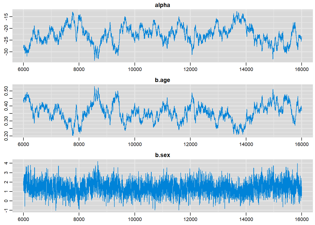
# Density plots
denplot(output, parms=c("alpha", "b.age", "b.sex"))
# Summary statistics
summary(output)
Iterations = 6001:16000
Thinning interval = 1
Number of chains = 1
Sample size per chain = 10000

1. Empirical mean and standard deviation for each variable,
   plus standard error of the mean:

            Mean       SD  Naive SE Time-series SE
alpha  -22.60139 3.768209 3.768e-02      0.7020891
b.age    0.35682 0.058783 5.878e-04      0.0107935
b.sex    1.39529 0.713802 7.138e-03      0.0271795
p[1]     0.96056 0.027404 2.740e-04      0.0034678
p[2]     0.30493 0.097055 9.705e-04      0.0037275
p[3]     0.63030 0.102256 1.023e-03      0.0016067
p[4]     0.24604 0.096675 9.667e-04      0.0047334
p[5]     0.96056 0.027404 2.740e-04      0.0034678
p[6]     0.99160 0.008695 8.695e-05      0.0013515
p[7]     0.47128 0.119090 1.191e-03      0.0023186
p[8]     0.82657 0.077578 7.758e-04      0.0037488
p[9]     0.55505 0.117898 1.179e-03      0.0021793
p[10]    0.03213 0.025665 2.567e-04      0.0034851
p[11]    0.54827 0.107063 1.071e-03      0.0015826
p[12]    0.38093 0.104193 1.042e-03      0.0019521
p[13]    0.99813 0.002661 2.661e-05      0.0003860
p[14]    0.23854 0.087435 8.744e-04      0.0048835
p[15]    0.10360 0.054984 5.498e-04      0.0052459
p[16]    0.97129 0.022743 2.274e-04      0.0025935
p[17]    0.23854 0.087435 8.744e-04      0.0048835
p[18]    0.98454 0.014339 1.434e-04      0.0016898
p[19]    0.94673 0.035503 3.550e-04      0.0033916
p[20]    0.08024 0.049191 4.919e-04      0.0050080
p[21]    0.90138 0.051118 5.112e-04      0.0048127
p[22]    0.07690 0.045483 4.548e-04      0.0049114
p[23]    0.99662 0.004277 4.277e-05      0.0006452
p[24]    0.90238 0.053846 5.385e-04      0.0041053
p[25]    0.86918 0.065176 6.518e-04      0.0040603
p[26]    0.99543 0.005421 5.421e-05      0.0008152
p[27]    0.98446 0.013878 1.388e-04      0.0020598
p[28]    0.03213 0.025665 2.567e-04      0.0034851
p[29]    0.96056 0.027404 2.740e-04      0.0034678
p[30]    0.46352 0.107739 1.077e-03      0.0016346
p[31]    0.98858 0.010995 1.099e-04      0.0016773
p[32]    0.98864 0.011347 1.135e-04      0.0013887
p[33]    0.05932 0.039925 3.992e-04      0.0045811
p[34]    0.98864 0.011347 1.135e-04      0.0013887
p[35]    0.94628 0.034034 3.403e-04      0.0041410
p[36]    0.70528 0.094104 9.410e-04      0.0030751
p[37]    0.08024 0.049191 4.919e-04      0.0050080
p[38]    0.82657 0.077578 7.758e-04      0.0037488
p[39]    0.97109 0.021933 2.193e-04      0.0029740
p[40]    0.54827 0.107063 1.071e-03      0.0015826
p[41]    0.63580 0.111968 1.120e-03      0.0020877
p[42]    0.18311 0.076562 7.656e-04      0.0056644
p[43]    0.55505 0.117898 1.179e-03      0.0021793
p[44]    0.97894 0.018084 1.808e-04      0.0020259
p[45]    0.24604 0.096675 9.667e-04      0.0047334
p[46]    0.92704 0.041932 4.193e-04      0.0045678
p[47]    0.31306 0.107493 1.075e-03      0.0039695
p[48]    0.86918 0.065176 6.518e-04      0.0040603
p[49]    0.97894 0.018084 1.808e-04      0.0020259
p[50]    0.94628 0.034034 3.403e-04      0.0041410
p[51]    0.94673 0.035503 3.550e-04      0.0033916
p[52]    0.97881 0.017476 1.748e-04      0.0024961
p[53]    0.04370 0.032117 3.212e-04      0.0040090
p[54]    0.07690 0.045483 4.548e-04      0.0049114
p[55]    0.13849 0.065493 6.549e-04      0.0059531
p[56]    0.04183 0.030139 3.014e-04      0.0038086
p[57]    0.97894 0.018084 1.808e-04      0.0020259
p[58]    0.18963 0.084359 8.436e-04      0.0052539
p[59]    0.86771 0.061459 6.146e-04      0.0053494
p[60]    0.54827 0.107063 1.071e-03      0.0015826
p[61]    0.54827 0.107063 1.071e-03      0.0015826
p[62]    0.30493 0.097055 9.705e-04      0.0037275
p[63]    0.01735 0.016173 1.617e-04      0.0023865
p[64]    0.01735 0.016173 1.617e-04      0.0023865
p[65]    0.47128 0.119090 1.191e-03      0.0023186
p[66]    0.30493 0.097055 9.705e-04      0.0037275
p[67]    0.99861 0.002099 2.099e-05      0.0002997
p[68]    0.07690 0.045483 4.548e-04      0.0049114
p[69]    0.63580 0.111968 1.120e-03      0.0020877
p[70]    0.94673 0.035503 3.550e-04      0.0033916
p[71]    0.99861 0.002099 2.099e-05      0.0002997
p[72]    0.98858 0.010995 1.099e-04      0.0016773
p[73]    0.99543 0.005421 5.421e-05      0.0008152
p[74]    0.99383 0.007079 7.079e-05      0.0009285
p[75]    0.70948 0.102290 1.023e-03      0.0020652
p[76]    0.01735 0.016173 1.617e-04      0.0023865
p[77]    0.99543 0.005421 5.421e-05      0.0008152
p[78]    0.99381 0.006869 6.869e-05      0.0010799
p[79]    0.70948 0.102290 1.023e-03      0.0020652
p[80]    0.97894 0.018084 1.808e-04      0.0020259
p[81]    0.99164 0.008966 8.966e-05      0.0011652
p[82]    0.90238 0.053846 5.385e-04      0.0041053
p[83]    0.92704 0.041932 4.193e-04      0.0045678
p[84]    0.01735 0.016173 1.617e-04      0.0023865
p[85]    0.90238 0.053846 5.385e-04      0.0041053
p[86]    0.97881 0.017476 1.748e-04      0.0024961
p[87]    0.97881 0.017476 1.748e-04      0.0024961
p[88]    0.99160 0.008695 8.695e-05      0.0013515
p[89]    0.97129 0.022743 2.274e-04      0.0025935
p[90]    0.54827 0.107063 1.071e-03      0.0015826
p[91]    0.14389 0.071796 7.180e-04      0.0054550
p[92]    0.18311 0.076562 7.656e-04      0.0056644
p[93]    0.63030 0.102256 1.023e-03      0.0016067
p[94]    0.86771 0.061459 6.146e-04      0.0053494
p[95]    0.02361 0.020410 2.041e-04      0.0029068
p[96]    0.94628 0.034034 3.403e-04      0.0041410
p[97]    0.99381 0.006869 6.869e-05      0.0010799
p[98]    0.07690 0.045483 4.548e-04      0.0049114
p[99]    0.10360 0.054984 5.498e-04      0.0052459
p[100]   0.97109 0.021933 2.193e-04      0.0029740

2. Quantiles for each variable:

             2.5%        25%       50%       75%     97.5%
alpha  -29.835282 -25.032849 -22.68508 -20.13662 -15.19306
b.age    0.240710   0.318278   0.35801   0.39473   0.47041
b.sex    0.039709   0.906206   1.37318   1.87335   2.83306
p[1]     0.889674   0.948991   0.96806   0.97971   0.99217
p[2]     0.138898   0.235284   0.29809   0.36732   0.51146
p[3]     0.415625   0.563690   0.63563   0.70347   0.81283
p[4]     0.092644   0.174542   0.23443   0.30588   0.46291
p[5]     0.889674   0.948991   0.96806   0.97971   0.99217
p[6]     0.967928   0.989416   0.99451   0.99707   0.99919
p[7]     0.249477   0.385631   0.47008   0.55398   0.70556
p[8]     0.649866   0.779622   0.83769   0.88525   0.94353
p[9]     0.325367   0.471722   0.55772   0.63957   0.77630
p[10]    0.004954   0.014377   0.02447   0.04201   0.10231
p[11]    0.333708   0.476150   0.55087   0.62307   0.74869
p[12]    0.191893   0.307751   0.37742   0.45026   0.59201
p[13]    0.990489   0.997861   0.99908   0.99958   0.99992
p[14]    0.097114   0.174509   0.22912   0.29319   0.43353
p[15]    0.029547   0.062710   0.09282   0.13199   0.24048
p[16]    0.909437   0.962905   0.97753   0.98709   0.99557
p[17]    0.097114   0.174509   0.22912   0.29319   0.43353
p[18]    0.944585   0.980343   0.98888   0.99403   0.99821
p[19]    0.854476   0.930314   0.95515   0.97253   0.98939
p[20]    0.018357   0.044460   0.06825   0.10410   0.20427
p[21]    0.774017   0.874011   0.91160   0.93876   0.97126
p[22]    0.019312   0.043477   0.06680   0.09874   0.19342
p[23]    0.984512   0.995929   0.99812   0.99908   0.99979
p[24]    0.770369   0.872952   0.91266   0.94291   0.97501
p[25]    0.712861   0.831446   0.88025   0.91877   0.96211
p[26]    0.980234   0.994402   0.99731   0.99866   0.99967
p[27]    0.947052   0.980065   0.98889   0.99360   0.99796
p[28]    0.004954   0.014377   0.02447   0.04201   0.10231
p[29]    0.889674   0.948991   0.96806   0.97971   0.99217
p[30]    0.256344   0.389227   0.46284   0.53651   0.67371
p[31]    0.958516   0.985453   0.99219   0.99566   0.99871
p[32]    0.956454   0.985692   0.99221   0.99594   0.99885
p[33]    0.011929   0.030725   0.04870   0.07768   0.16250
p[34]    0.956454   0.985692   0.99221   0.99594   0.99885
p[35]    0.859402   0.930558   0.95493   0.97053   0.98789
p[36]    0.500585   0.644955   0.71262   0.77367   0.86539
p[37]    0.018357   0.044460   0.06825   0.10410   0.20427
p[38]    0.649866   0.779622   0.83769   0.88525   0.94353
p[39]    0.914056   0.962680   0.97747   0.98616   0.99499
p[40]    0.333708   0.476150   0.55087   0.62307   0.74869
p[41]    0.407257   0.558304   0.64239   0.71810   0.83434
p[42]    0.066411   0.126006   0.17210   0.22861   0.35830
p[43]    0.325367   0.471722   0.55772   0.63957   0.77630
p[44]    0.928567   0.973023   0.98423   0.99119   0.99716
p[45]    0.092644   0.174542   0.23443   0.30588   0.46291
p[46]    0.821579   0.906170   0.93669   0.95729   0.98135
p[47]    0.132648   0.233989   0.30434   0.38266   0.54416
p[48]    0.712861   0.831446   0.88025   0.91877   0.96211
p[49]    0.928567   0.973023   0.98423   0.99119   0.99716
p[50]    0.859402   0.930558   0.95493   0.97053   0.98789
p[51]    0.854476   0.930314   0.95515   0.97253   0.98939
p[52]    0.932602   0.972665   0.98411   0.99059   0.99678
p[53]    0.007691   0.021151   0.03464   0.05714   0.12886
p[54]    0.019312   0.043477   0.06680   0.09874   0.19342
p[55]    0.044540   0.089458   0.12674   0.17461   0.29532
p[56]    0.008180   0.020577   0.03360   0.05409   0.12355
p[57]    0.928567   0.973023   0.98423   0.99119   0.99716
p[58]    0.063680   0.126796   0.17721   0.23953   0.38532
p[59]    0.719891   0.833258   0.87859   0.91290   0.95673
p[60]    0.333708   0.476150   0.55087   0.62307   0.74869
p[61]    0.333708   0.476150   0.55087   0.62307   0.74869
p[62]    0.138898   0.235284   0.29809   0.36732   0.51146
p[63]    0.002036   0.006677   0.01218   0.02228   0.06328
p[64]    0.002036   0.006677   0.01218   0.02228   0.06328
p[65]    0.249477   0.385631   0.47008   0.55398   0.70556
p[66]    0.138898   0.235284   0.29809   0.36732   0.51146
p[67]    0.992594   0.998448   0.99936   0.99972   0.99995
p[68]    0.019312   0.043477   0.06680   0.09874   0.19342
p[69]    0.407257   0.558304   0.64239   0.71810   0.83434
p[70]    0.854476   0.930314   0.95515   0.97253   0.98939
p[71]    0.992594   0.998448   0.99936   0.99972   0.99995
p[72]    0.958516   0.985453   0.99219   0.99566   0.99871
p[73]    0.980234   0.994402   0.99731   0.99866   0.99967
p[74]    0.973218   0.992459   0.99621   0.99813   0.99954
p[75]    0.493526   0.642486   0.71855   0.78575   0.88221
p[76]    0.002036   0.006677   0.01218   0.02228   0.06328
p[77]    0.980234   0.994402   0.99731   0.99866   0.99967
p[78]    0.974838   0.992289   0.99616   0.99801   0.99948
p[79]    0.493526   0.642486   0.71855   0.78575   0.88221
p[80]    0.928567   0.973023   0.98423   0.99119   0.99716
p[81]    0.965857   0.989593   0.99458   0.99724   0.99927
p[82]    0.770369   0.872952   0.91266   0.94291   0.97501
p[83]    0.821579   0.906170   0.93669   0.95729   0.98135
p[84]    0.002036   0.006677   0.01218   0.02228   0.06328
p[85]    0.770369   0.872952   0.91266   0.94291   0.97501
p[86]    0.932602   0.972665   0.98411   0.99059   0.99678
p[87]    0.932602   0.972665   0.98411   0.99059   0.99678
p[88]    0.967928   0.989416   0.99451   0.99707   0.99919
p[89]    0.909437   0.962905   0.97753   0.98709   0.99557
p[90]    0.333708   0.476150   0.55087   0.62307   0.74869
p[91]    0.042420   0.090691   0.13080   0.18464   0.31761
p[92]    0.066411   0.126006   0.17210   0.22861   0.35830
p[93]    0.415625   0.563690   0.63563   0.70347   0.81283
p[94]    0.719891   0.833258   0.87859   0.91290   0.95673
p[95]    0.003212   0.009801   0.01724   0.03062   0.08035
p[96]    0.859402   0.930558   0.95493   0.97053   0.98789
p[97]    0.974838   0.992289   0.99616   0.99801   0.99948
p[98]    0.019312   0.043477   0.06680   0.09874   0.19342
p[99]    0.029547   0.062710   0.09282   0.13199   0.24048
p[100]   0.914056   0.962680   0.97747   0.98616   0.99499
Hierarchical Binomial Proportion
modelString =
  "model { for (i in 1:nmd) {                  #  nmd = number of MDs participating
        x[i] ~ dbin(p[i],n[i])          #  likelihood function for data for each MD

       logit(p[i]) <- z[i]              #  Logit transform
        z[i] ~ dnorm(mu,tau)            #  Logit of probabilities follow normal distribution
      }

           mu ~   dnorm(0,0.001)        # Prior distribution for mu
          tau ~   dgamma(0.001,0.001)   # Prior distribution for tau
          y   ~   dnorm(mu, tau)        #  Predictive distribution for rate
        sigma <-  1/sqrt(tau)           #  SD on the logit scale
            w <-  exp(y)/(1+exp(y))     #  Predictive dist back on p-scale
  }"

#Write the model to a file
writeLines(modelString,con="model.txt")

#Compiling the model together with the data
jagsModel = jags.model("model.txt",list(n=c( 20, 6, 24, 13, 12, 4, 24, 12, 18),
                                        x=c( 19, 5, 22, 12, 11, 4, 23, 12, 16),
                                        nmd=9), list(mu=0, tau=1))
Compiling model graph
Resolving undeclared variables
Allocating nodes
Graph information:
Observed stochastic nodes: 9
Unobserved stochastic nodes: 12
Total graph size: 48
Initializing model#Burn-in
update( jagsModel,n.iter=5000)
# The parameter(s) to be monitored.
parameters = c("mu", "tau", "sigma", "w", "y", "p")
#Sampling from the posterior distribution
output = coda.samples(jagsModel,variable.names=parameters,n.iter=10000)
# Examining the posterior sample
# History plots
traplot(output, parms=c("sigma", "w"))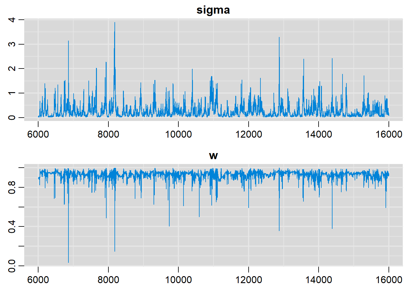
# Density plots
denplot(output, parms=c("sigma", "w"))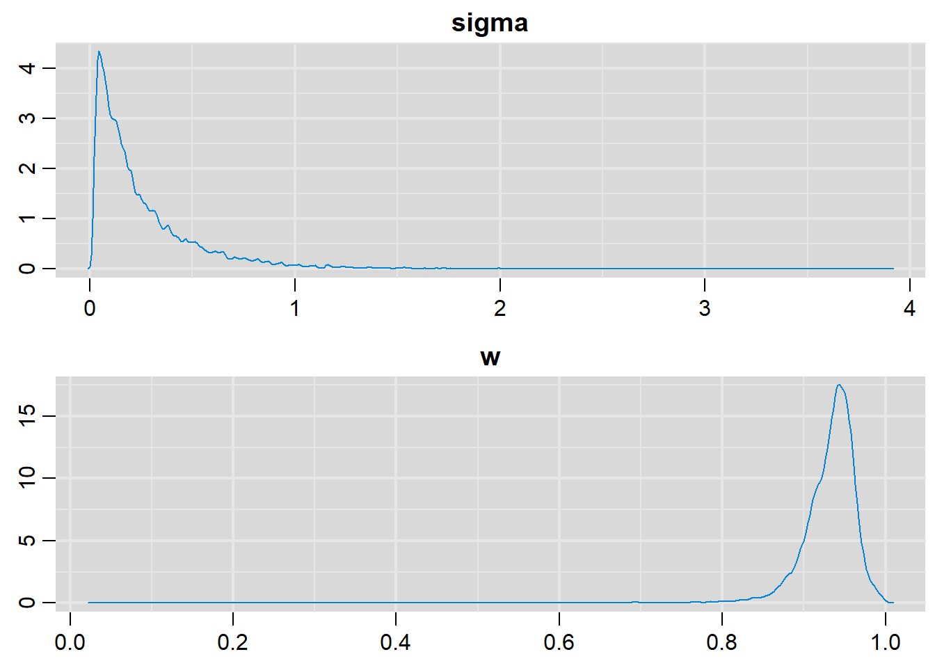
# Summary statistics
summary(output)
Iterations = 6001:16000
Thinning interval = 1
Number of chains = 1
Sample size per chain = 10000

1. Empirical mean and standard deviation for each variable,
   plus standard error of the mean:

          Mean        SD  Naive SE Time-series SE
mu      2.7077   0.36042 0.0036042       0.026017
p[1]    0.9343   0.02543 0.0002543       0.001512
p[2]    0.9272   0.03586 0.0003586       0.001895
p[3]    0.9310   0.02742 0.0002742       0.001583
p[4]    0.9316   0.02888 0.0002888       0.001532
p[5]    0.9321   0.02765 0.0002765       0.001427
p[6]    0.9332   0.02982 0.0002982       0.001630
p[7]    0.9355   0.02479 0.0002479       0.001631
p[8]    0.9368   0.02600 0.0002600       0.001734
p[9]    0.9286   0.02991 0.0002991       0.001562
sigma   0.2618   0.28083 0.0028083       0.017486
tau   179.4206 396.26260 3.9626260      17.689896
w       0.9311   0.03747 0.0003747       0.001496
y       2.7122   0.52561 0.0052561       0.025850

2. Quantiles for each variable:

         2.5%     25%     50%      75%     97.5%
mu    2.01512 2.45516  2.7137   2.9414    3.4214
p[1]  0.87590 0.92015  0.9383   0.9517    0.9750
p[2]  0.83760 0.91413  0.9354   0.9495    0.9710
p[3]  0.86566 0.91690  0.9363   0.9497    0.9710
p[4]  0.86565 0.91693  0.9371   0.9506    0.9733
p[5]  0.86739 0.91775  0.9371   0.9509    0.9741
p[6]  0.86705 0.91833  0.9384   0.9525    0.9785
p[7]  0.87635 0.92124  0.9395   0.9528    0.9757
p[8]  0.87667 0.92244  0.9407   0.9540    0.9811
p[9]  0.85670 0.91443  0.9349   0.9489    0.9691
sigma 0.02726 0.08141  0.1691   0.3381    1.0003
tau   0.99948 8.74990 34.9918 150.8721 1346.1070
w     0.85654 0.91696  0.9377   0.9519    0.9776
y     1.78688 2.40174  2.7106   2.9843    3.7782
Citation
BibTeX citation:
@online{yao2020,
  author = {Mandy Yao and Nandini Dendukuri},
  title = {Learning Rjags Using Simple Statistical Models},
  date = {2020-07-25},
  url = {https://www.nandinidendukuri.com/blogposts/2020-07-25-simple-rjags-models/},
  langid = {en}
}
For attribution, please cite this work as:
Mandy Yao, and Nandini Dendukuri. 2020. “Learning Rjags Using
Simple Statistical Models.” July 25, 2020. https://www.nandinidendukuri.com/blogposts/2020-07-25-simple-rjags-models/.